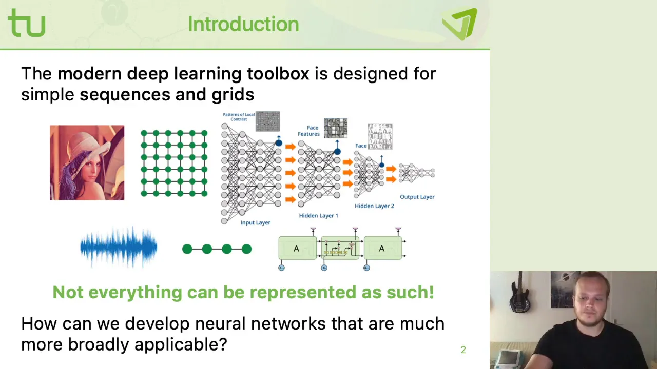
Geometric Deep Learning: Graph Convolutional Networks Tutorial

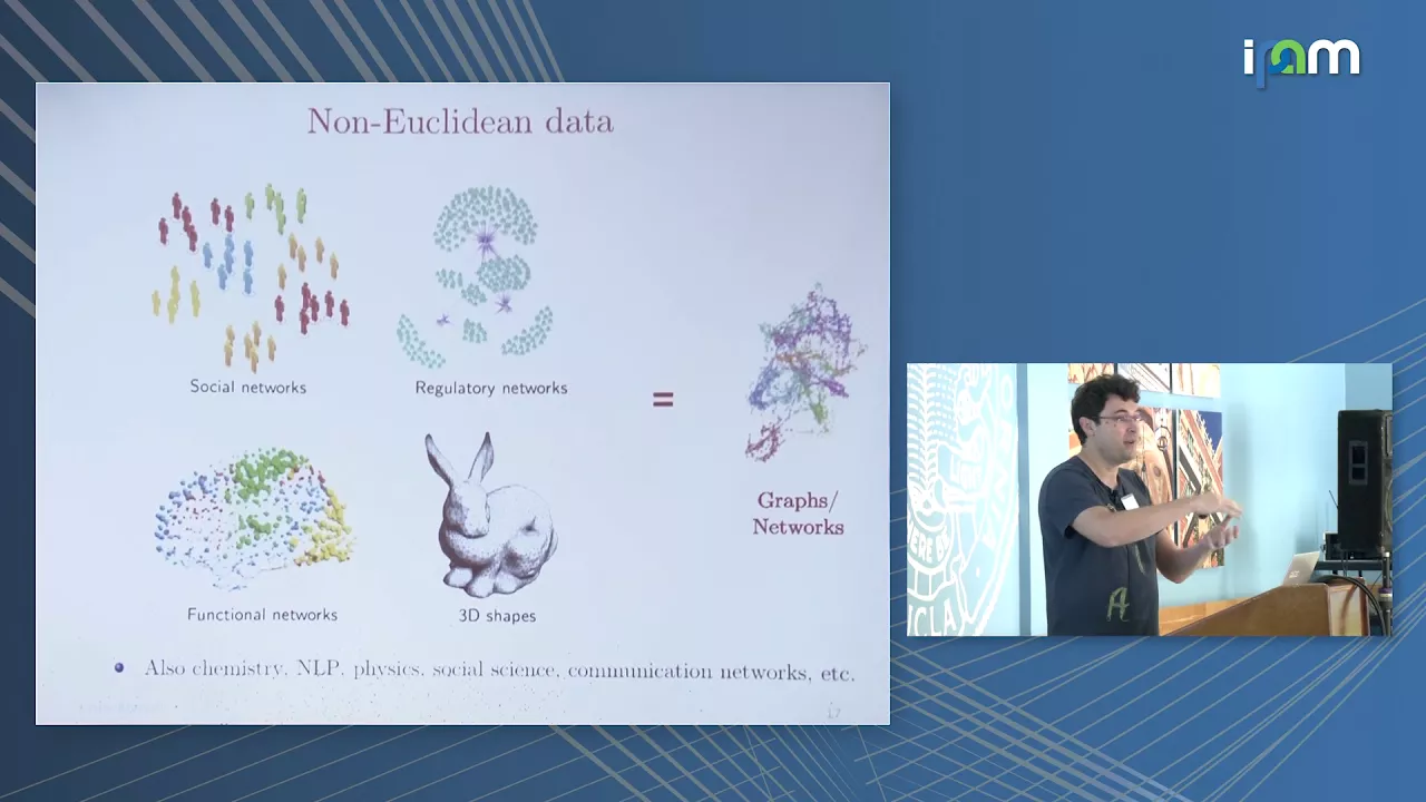
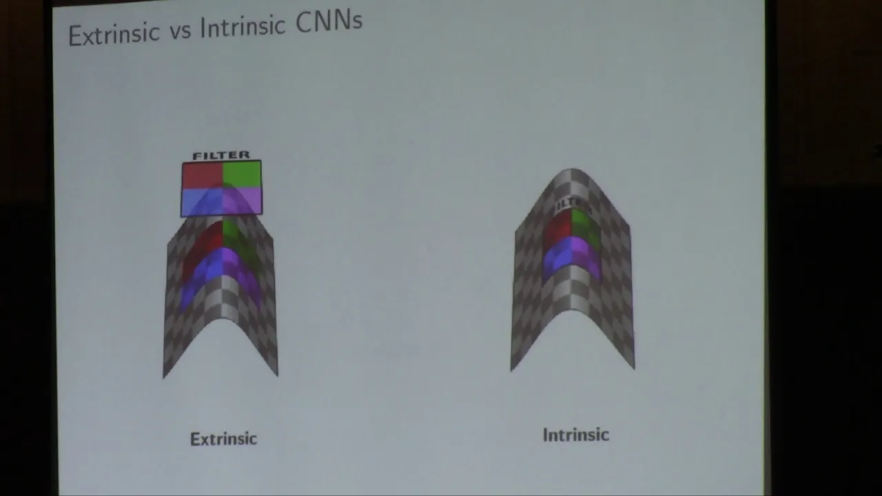
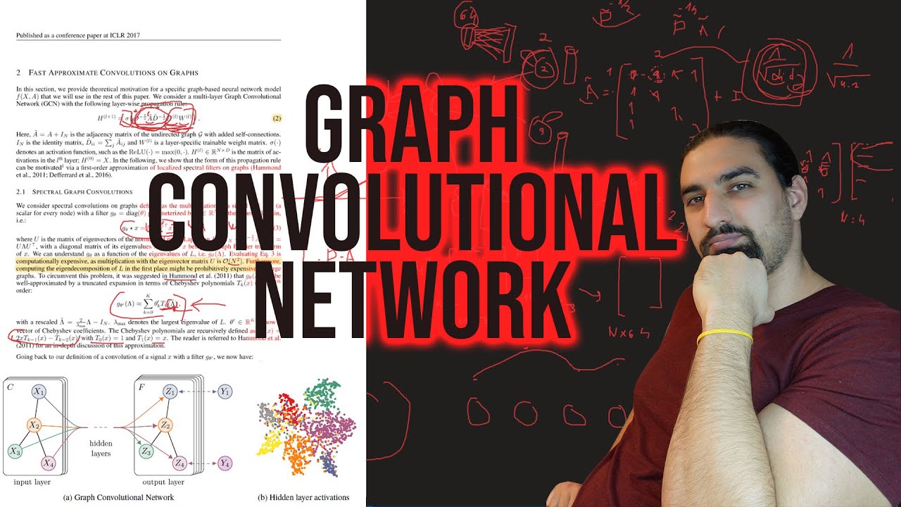
[00:00:00]let's let's begin today we're talking about geometric deep learning it's a pretty new and hot topic these days and we'll kind of show it a bit and give a small taste of it will specifically we'll cover how to do filtering on graphs and show what graph laplacian czar and define a graph convolutional layer based on things that we that you you have seen in the video lectures and will then implement a small application example of node classification in a graph classifying nodes in a in a given graph ok so first let's remind ourselves the the required theory that we need for today's application alright so we we've seen convolutional layers a lot in this course and if you remember a convolutional layer operates on feature maps the feature maps usually were 2d sometimes it can be 1d as we already saw so so you have the this feature map then you have some filter and you do a convolution between the filter and each each your map and then you sum over the future maps to create the output feature map so in case of images we had these 3d filters that were spatially local and they were summing over all the input channels this is just another way to write it and this star operator denotes the convolution so we like these layers because of the advantages that they provided namely the the number of parameters was small it isn't did not depend on the input dimensions and there was parameter sharing which is a useful property and as we saw in CN NS the output dimension changes based on the input so today we'll kind of try to define something similar to these these layers for data that lives on graphs and does not live on on regularly Lydian domains so where this convolution operator is not valid okay so let's just briefly write ourselves what so basically if you want to convo functions you sum the product of those functions well the definition is that one of the functions should be flipped and you sum them point wise basically a small caveat here is that actually in cnn's the the operation that they perform is its correlation not convolution they don't directly flip anything but this is just the formal definition of a convolution and as you know this is a linear operator and any linear operator can be represented as a matrix multiplication and specifically the revolutions are represented as topless matrices where the these ABC and these are the filter the filter parameters you have this matrix which if the filtering this represents the convolution operator if you take this matrix and multiply it by some vector which represents a discreet function okay and it's shifter covariance which means that if you provide a shift to the input your output will be shifted by the same amount right so so from linear algebra we know this concept of an eigen decomposition which allows attitude allows us to diagonal matrix and an interesting property that we will use here is that all these top --let's operators have the same eigen vector vectors which is a useful property and this this is the basis or these are the eigenvectors you can define them like that we define in using these this notation of a discrete harmonic which here we define on on a discrete spatial coordinate so this you can imagine this is just one D okay so this could be a one d in space and in in frequency it's continuous okay so if you actually want to see that that these are the eigen eigen functions of the top of an Tablas operator if you have some topless matrix and you multiply it by this vector so here this is sorry so this is a factor we remove the n here so this is a vector of all the N locations of this discrete harmonic and we're looking at the enth output and since it's a topless we can write it as a convolution and then we just use the definition of the convolution and since this is an exponent you can split it and basically what you get is the is this discrete harmonic times the inner product between your filter vector and that vector that you you input here okay so shows that this is a an eigen a an eigen vector of the matrix so basically that's that's the the idea so any any of these discrete harmonic see here again this is a vector for all the ends in a specific frequency C so you get this these eigenvectors eigenvalues sorry okay so we're gonna need this property and since this is a Fourier basis we just can say this is also a Fourier transform if you take the inner product between some vector and this sorry again between some vector and this and this I can vector you get the coordinates which represents the coordinate of the Fourier transform same for the inverse transform here the inner product is an integral because the domain here is a continuous so that's basically the idea and the use of property that we're gonna need to define the graph the graph convolution later layer which will implement later on is the fact that if you have a time a convolution in time domain just exactly by using the definitions that I saw that I shown in the previous slide you can just plug this in and write it write the convolution as a topless matrix times your vector and then you can write this vector as a Fourier transform and then an inverse Fourier transform so inner product here and then the outer inner product on the continuous domain is the integral and then you move the matrix inside and then here you have the matrix times an eigen vector so you get an eigen value of the matrix okay and this actually now in the frequency domain this is an inner product between these two vectors and this vector so basically the point is that in the you can say time domain convolution is frequency domain multiplication between the representations so this this is also known as the Constitution theorem this is what we will use later on this this yeah this is to please yeah we just write that right these coefficients in the top list matrix and then it's an operator that we can apply to a vector okay so let's talk about graphs so so graphs are generally enough to represent other non Euclidean amines like like point clouds or manifolds so it's it's an interesting domain to look at and see how we can represent functions on graphs and what we can do with them with deep learning so I'm sure you in your studies here already seen lots of graphs but we have this graph defined by a vertex set or also known as nodes so you have n nodes here you have edges between each two nodes possibly generally you have a vertex weight so weight for each of the vertices represent it as a diagonal matrix and usually what we care about is this edge weight so it's an adjacency matrix which just gives you the weight between node imj where if they're not connected then the weight is just 0 so you have a matrix representing the graph and if you have vertex weights you have another matrix representing them okay so that's a graph what what is a signal on a graph so a vertex signal just or a function on a graph you just can define it as this vector okay so if you have n nodes it's just a vector with n elements corresponding to the function to the value of the function at each of those nodes that's it and we can define this this space with an inner product inner product space between two functions on the graph again these are detectors now if it's a since we're talking about the graph which is discrete and the only difference is it's a regular product but we have to wait it by the way these vertex weights okay so the important thing here is that we the function on the graph is just a vector okay and similarly we can define a function on the edges but it's not relevant for today so okay so the next thing that we need for our graph convolution network is the laplacian of the graph so the plasma of the graph is an operator you can apply it to a function on a graph and you get another vector so you apply it to one vector representing a function when you get another vector and it's actually a measure of smoothness it's it tells you how if you apply this laplacian what you get out is the measure of how smooth the function on the graph is how quickly it changes between nodes node to node when we're talking about adjacent nodes okay so formally you you are you define it from again from the space of functions on nodes to space of functions if you look at the laplacian of some function on a graph at point I so the at the ice node or the output of the laplacian on f looking at the i coordinate what you see is it's basically it's a it's a weighted difference where you take the value of the function at node I and subtract the weighted sum of the of the function value around node I yeah the neighbors direct neighbors that's why that's what the J naught equals I here means and W IJ is the adjacency okay so it gives you the weighted sum of the function value between a node and all its neighbors yes okay so again if the function changes quickly from node to node then a plus sign will have a high value if it changes slowly from node to node you have an over W yeah W it can be binary that means the weights are all equal to 0 1 or it can be continuous yeah okay so that's the laplacian and usually we refer it san operator we can represent it as a matrix so if you have this laplacian matrix you just multiply this matrix by a vector representing a function on the graph what you get is the output of the laplacian for each node in the graph so usually this is how it's defined DD minus W in with this scaning so there's lots of different definitions which are similar for the laplacian so we're going to use one of the one of the definitions that that's similar to that the next thing that we need is to take the graph laplacian and look at its eigen values or vectors okay so in the so this is also an example the there's also a plus sign in the regular plus in for functions in the including domain and it's also a translation equivalent operator and also has a free eigenbasis so you can really see it easily if you just take this of this harmonic function take it it's a laplacian just by definition the sum of the second derivatives and you can see you get the same function scaled by this eigen value okay so same idea now just we have a laplacian on a non Euclidean domain but we'll just do the same thing we'll take the eigen decomposition of our laplacian matrix and say that this is now a basis to represent functions on the graph okay that's the idea so the laplacian has an eigen decomposition will write it as this fee matrix okay so this is the matrix with eigenvectors in the columns and lambda is the diagonal matrix of eigenvalues of the laplacian matrix if you have if you have vertex weight then then you have a orphan or wrong which which means that it's also normal if you put a here then you get AI but usually in our example we'll also ignore this aim all our edges will have the all our nodes will have the same way okay so now we have an eigen decomposition let's look at what it means so the the interesting thing is that these eigenfunctions of the laplacian or the eigenvectors in our case which is discrete or are again there are functions on the graph they have the vectors with n elements and they represent the smoothest possible basis functions so you can represent another function using a linear combination of these functions and they represent a very smooth basis so if you look for example the euclidean remain the Fourier basis is these sines okay so you have first a constant and then a low frequency and goes to higher frequencies and if you look at the laplacian eigenvectors of other kinds of domains like manifold or the graphs which is a discretization of that you can see kind of the first eigen function which is a constant and the second one is something that changes slowly so as you go to higher I gain functions or in the case of a graph I gain factors it represents a function that changes quickly on the graph higher frequencies okay so again we'll look at that soon and again since this is a basis for this space of functions on the graph we can represent any function on the graph as a linear combination so let's say I have some function on the graph I can write it as a linear combination of my eigen vectors and the coordinate the scalar that I need to to multiply here is just you computed by the projection this inner product with from between my function and this eigen vector okay so this basically in your honor and based on that again from similarly since we saw this is a Fourier basis we can say that this is a Fourier transform if you take if you take your function and transfer using these eigenvectors of the laplacian so you can define the free trade zone and the backward fringes from this way and now finally with all of that we can define convolution layer for graph so you'll see two versions one is the spectral version which is directly based on this definition and you'll see that it has drawback so we can't really implement it efficiently and then we'll see the the improved version which we can implement and then we'll implement it and look see what happens okay so we saw the convolution theorem in the Euclidian case if you take your filter topless matrix you can say it's a convolution in time okay but in frequency it's you can you can say it's in frequency it's a multiplication so this is just based on the definitions that we saw okay exactly this is exactly dragged from the definitions now in the non-league Lydian domain since our our function is on a graph we can't really move it around it does it doesn't mean anything to shift it when we want to compute the convolution because again our function is just value a value for each node on the graph so there's no meaning but but but what we can say now is that instead of doing this convolution part we'll just skip it just skip this part of the equation so we'll define the this operator as the inverse Fourier transform of the multiplication in the frequency domain of the of our function okay so we want to compute the convolution with this function but what we'll do is we'll just skip this middle part and define it this way and again like we saw we have we know how to compute this this Fourier transform based on the eigen vectors of the laplacian so now we can just define it like that directly and we say this is the definition of convolution on a graph this we just define it this way okay here it it was derived from our our formulas but here we just defined like that and you can see that what you get is two you get this expression you just plug everything in you take your f you compute basically the inverse the Fourier transform here by this multiplication then you you apply diagonal matrix which represents the filter in the frequency domain and then you do the inverse Fourier transform to get it back to the original domain that's the interpretation here so again W is the diagonal matrix representing filter parameters so since we're in a deep learning course we'll want to learn the filter parameters and this is basically the first definition of a graph CNN okay so we can define the spectral version of a graph CNN this way so now if we have our features so we have now we have M features for each vertex okay so we'll think about it as as feature Maps so you have for all of the nodes you have any feature Maps yet because you have M M features for each node so this is our X this is our feature Maps and the output should also be feature Maps with a different number of feature Maps just like a CNN where you take future Maps do the do the CNN layer and then you get output feature Maps and we define it based on the previous slide formula you take your input feature map so this is a vector representing a function on a graph you do this space spectral part where you take the Fourier transform apply the filter reverse Fourier transform and then you get you you sum it on all the feature reps to combine between feature maps again like a CNN and then you get your output feature map this is a J's feature yes it's a vector no it's a vector of length n representing the value for each node so let's say so let's look at X so X would be a matrix with 1 to n here and this is the first feature map this is the second feature so I have M feature maps ok so this is so for if you look at a specific node then for specific node you have M features for that node all right so but this actually is problematic so if you remember from the lecture Alex talked about this abit why why is this the finish not actually very useful why isn't that useful to define a scene on a graph so we have our data it lives on a graph we know what everything he represents so this is the features on a graph it's great but why can't we actually use this no why why is this not something that we would like to implement what's the drawbacks ok so the multiple drawbacks here first of all it's you have to compute this matrix multiplication with an N by n matrix twice once here once here second the number of parameters remember this is a diagonal matrix of length of size n so we have n parameters and n is the number of nodes in your graph ok so it's not like a convolutional layer where the number of parameters is fixed and not dependent on the spatial extent of the image it's not so it's not really very useful and there's another issue with fact that you're using the the highest eigen vectors which represent high frequency functions so you you you might insert high frequencies and the reason that that's that's not very useful or less less desired if you recall from the lecture Alex showed why there's this connection between smoothness in frequency and spatial localization so you will get non spatially localized so special localization in the graph means the operation is operates on a node and it's close neighbors so you you will not have that ok so these are the basic drawbacks of this method ok so just as an example the last one the last last the last drawback is also interesting if these are learned parameter they depend on this fee they will depend on what exactly your fee was and the fee depends on the graph structure because it's based on the adjacency matrix so you will have a different fee for each graph and so another problem is that if you move to a different graph your learned filter will not generalize okay so it's kind of hard to imagine but here's a here's a nice example that shows that so let's say we have this manifold so it's like you can think about this continuous conversion or a graph could be a discrete version of this and you have some function f which which is represented by the red parts here so you have a function on a manifold and here you apply some filter W on your function and in this case it looks like an edge detection filter you can see it really detects the edges of function but if you have a different manifold which is actually not deform just you just moved move the manifold it's an isometry then you have a completely different meaning of your filter now so you applied here the same W but you have a different fee okay so this would correspond to a graph where I changed the adjacency matrix okay so now let's finally define what we need for our application today the spatial version of the conditioner so the spatial version is as the name suggests it's something that we want to do directly on the data in the spatial domain like as it is on the node without going through the Fourier transform in the back for interest okay so the way we do it is is this way we define our parameters so this is these are the N parameters from our W matrix our diagonal W matrix as we define them as linear combinations of some functions of the eigenvalues of the laplacian again so now our parameters will be these these q parameters of course we have a parameter for each input and output feature now as usual in in every CNN case and these functions but better one to better cue are just some smoosh functions we'll see an example of polynomials and there's lots of different kinds of phone numbers that are used okay so now because it's defined like that the number of parameters does not is not n anymore it does not depend on n the number of nodes so how many parameters do we now have and it is how many parameters learn about parameters we have q But Q for every input and output feature nope so we have Q times M times M prime so this is the input let's say in output teachers you'll see it by some definition and the second thing is that if you take polynomials as these betters then you can write it like like this your W matrix again so the W each W is a linear combination of the eigen with eigen values so if you're better is just regular polynomial then you have this on the diagonal then you can move out the sum and you get something very nice you get that it's lambda to the K and basically since this lambda this is an eigen decomposition of of the laplacian matrix it's equivalent to taking the case power of the laplace okay so you take the eigen decomposition and take the diagonal part to the case power so now we have something interesting so this whole four yeah ply filter and then inverse Fourier is equivalent to multiplying by the powers of the laplacian for this bit yeah it's a parameter its first corresponds to how you decide the filter size of your CN n it's hyper parameter set Q is a hyper parameter I guess it depends on the domain and your problem and finally now this is the spatial definition of the Fourier CN n layer so you can see now we have an an input feature map we multiply it by the laplacian or the case for the laplacian we do that for all the different case using this alpha and we have to sum over the input feature maps to combine the input feature maps and get one out could feature map okay so this is the definition that we'll use and since the laplacian if you remember represents a weighted sum of the function value between a node and its neighbors it's possible to show that the powers let's say the laplacian to the second power represents the it's an operation that's local in K in a k ring so it would represent the neighbors of the neighbors so it it depends on the value of the node and the value of the neighbors and the value of the neighbors neighbors but not anything beyond that so this is a local operation this is the power here of using a cousin and we'll see why this actually helps us solve our problem later on okay and there's no need to compute the eigen decomposition and there's no need to multiply by the Fourier and the inverse Fourier matrices okay so we'll write it a bit more generally like like so where we have X now again this is our data representing the M feature maps of our input and these this beta is some function that will take polynomial so there's lots of papers defining different betas and this is basically the final version that we're going to implement now so let's go our application today unless there's any questions about that will be to classify nodes in a given graph in a semi-supervised way which means we will only have the labels for two specific nodes and we'll try to classify the rest of the graph based on the connectivity and by implementing a graph convolutional layer okay so it's this approach here that I'm showing is based on the paper by Keefe and Welling from 2016 you can look at the paper we'll only have the true label for a tiny subset of the nodes in this case two nodes and we'll try to classify all the nodes okay so let's start with the data set we'll use a toy data set a very small graph known as the Zachary's karate club graph it's a network with two communities roughly communities which will try to classify each node as belonging to one of the communities in the graph and this is a based on some paper and topology paper from the 70s where the network the graph shows 34 members of a karate club and each node in the graph documents the fact that two people interacted outside the club right so they met each other maybe outside the club and at one point a conflict arose between the administrator of the club and the instructor the karate instructor so it led to a split of the club into two so about half of the members formed a new karate club around the instructor and the other people they just quit they either gave up karate or they found a new instructor somewhere else so basically we have two things that happen to the people of this club I want to predict what happened to the person based on the fact whether they interacted outside the club before the split all right so let's look at this we have I'm using this library called Network X it's useful library for working with graphs in Python and this is the famous example so they actually have this graph built in looking at the data I know the ID of the node representing the instructor and the idea of the node representing the administrator of the club okay and this is you can see a small graph only 34 vertices and 78 edges let's visualize the graph I'm using here again the sorry network X so this is just some code to visualize it you can see this is the administrator now this is the instructor node and the rest of the nodes correspond to the members so it's roughly it looks like roughly maybe there are two communities here in this graph but not every node this is not obvious completely where the affiliation would go just by looking at it visually okay so let's kind of see what we can do with this graph now first of all let's calculate its adjacency matrix just something I can do directly with this library and the degree matrix which is just summing the giant summing digesta see column wise because it will tell you how much how much connectivity how much how many nodes are connected to each node and then the laplacian just by definition D minus a in this case okay so let's calculate that so as you can see the adjacency matrix just in this case it's binary we don't have weight it just tells you whether in this case no the 1 is connected to 2 node 2 and laplacian is the degree minus minus a so the fact that we have 16 here shows that the this node 1 has 16 neighbors okay and finally we compute the eigen decomposition of the laplacian and we get the eigen values and eigen vectors here so few would be our vectors and this would be advanced we can just plot the eigen eigen values this is the spectrum of the opposite ok so just just to see what we're working with and another thing we can show is the the Fourier basis you know it's like that wait so here is um remember the the fee is the the eigen decomposition of the laplacian if we color the nodes based on so basically every column here is a function on a graph and remember that these are the smoothest functions this is a smoothest basis so if you color the graph according to the the values of these functions you should see that it's it becomes less smooth as you go to higher icon values so again smooth means the function value is changing quickly between nodes you can kind of see it very small graph but you can see these are less smooth functions here okay so that's that's nice but let's actually start implementing so now each each node in the graph has this extra attribute club which represents the members post split affiliation or what what group he joined after the split in the club so this will be our our labels but again will not use all the labels we'll save them for test time but will only train on the label of the instructor and the administrator okay and to just show that this is working based on the the connectivity of the graph itself we won't actually have any features here so our our matrix will just be an identity matrix our data matrix will just be an identity matrix okay which means that basically our only feature is the identity of the of the node and we will have to do all the predictions based on the connectivity of the graph if we had extra information we could we could have encoded the extra information here all right so here we just we create our X so this is our input matrix representing the for each node so each member each remember the features that we know about that member the labels are just based on this extra info you can see that for the nodes we have this data which is just uh just this dictionary that tells you what the post-split affiliation is so based on that I'm just computing the labels it should be 0 or 1 0 means they stayed with the instructor 1 means they left to a different instructor or left Crotty okay so in the paper they use a normalized version of the graph laplacian so we'll do the same thing they define the opacity in this way where D is the adjacency the degree matrix and a tilde is just a plus plus I okay so you can see instead of d- a they define it like that based on degree so this is one way to define a class since it's a valid definition and if you look at the elements of the Sebastien it's basically the idea Jason C normalized by the degree the products of do okay and since we added I we have these self loops and the what's the what's the point of having these self loops now if we would have defined it the plus in this way without adding this I what would happen try to imagine what the laplacian is doing remits local it's the local operation right so basically if if we wouldn't add at this I and define it like that then it would not allow the output features of a now to depend on the value of the node okay so the fact that we we add this we can you can also depend on the actual value of the node not just its neighbors so this is just the way that they finally they add a die and then normalize it this way okay and the model in the paper is defined in this in this way so for layer L what they do is they they have this this input feature maps for the layer L multiplied by the laplacian okay and then weighted by this output matrix to calculate the output feature Maps so so the inputs are n by M so this is the M is the input number of feature maps and M prime is the output number of feature maps so again think about this for a second what what does it mean what's going on in it is think about this part and this part separately so so this part is the laplacian times the feature maps so remember that the laplacian is a local operation it takes the value of a node weighted sum with its neighbors so what this part is doing it's it's combining local features in the same feature map okay and the second part the W is transforming across multiple feature mats and combining them to the output feature Maps like in like it as regular CNN where the output depends on all the input feature Maps you have you have a spatial region and you look at all the channels okay so you always look at all channels so this is exactly what's going on here this ensures you're you're using the information locally and then this allows you to do the linear combination to combine different feature Maps to get an output so this is the definition now I'm just implementing the adjacency matrix and adding this I and defining the laplacian based on their definition so it's a D to the minus half times a times e to the months okay so this is just what's going on here this is the laplacian definition from the paper the model is a graph convolution network based on the spatial version that we saw in the beginning and we'll compute simple powers of there plus and so we'll take beta as just regular polynomial functions right so if you want to visualize then we'll have a month with two graphs convolutional layers each layer takes a tensor with seeing seeing features for each node and represent gives you see out features so so you have a graph each node has see features which is represented here by this these rectangles so again for each node I have some number of features I'm applying my grass proposition layer and getting a different number of features and Prime okay and finally I will have labels for two nodes which I will use to compute the loss only from those two nodes and then back prop through that so this shows the idea and the way that we're going to Train okay so again remember the definition of the spatial GCN we have a feature map we apply the laplacian to some power and then we wait it using the weight matrix okay so this is a this already represents all the output feature maps and this represents all the input features okay and will implement it with a simple case of the better K is just equal to lambda to the K so let's look at the implementation finally we have some some code the gcn layer takes the graph laplacian so this first graph laplacian this just represents the graph this is all the information that we need to know about the graph input number of features output number of features for this layer and max dag is the mack the cue it's like you it's the maximal degree of the polynomial that we believe so remember we need to sum over these these Q's we have to we have to we have to sum until Q as you remember from here so this alpha K is just a linear layer just regular linear layer and the last one should have a bias also so we'll have F C fully connected layers so each FC layer is like the alpha K matrix okay so we just create these FC s from input features to output features with the last one having a bias and will also pre calculate the the beta K of the laplacian so we have this function here taking the replace ian i will just just calculate the laplacian times itself to get the powers of the laplacian and just save it in the in the forward pass we just directly implement the formula that you saw so we take X which represents the feature Maps for each node okay and we we just go over our our fully connected layers in K we take the case power of the laplacian multiply it by X okay and then apply a fully connected layer this is the multiplication with alpha where the last one has a bias so you'll get the bias here and then we sum them that's it Oh finally also we have a non-linearity and that's it that's the basically one graph convolutional layer the spatial version implemented again based on the given laplacian for a given graph okay so in our problem again we have this X that we created before using an identity matrix so the number of input features is the number of columns in X the number of output features is 2 because we're trying to predict whether the nodes belong to class 1 or class class 0 or class 1 this is the post bit affiliation so we have two output features the graph laplacian we calculated before based on the definition in the paper so just cut creating a tensor will define the maximal polynomial degree is two so we'll take powers of two of the laplacian and another hidden another hyper parameter we have is the hidden dimension so for now good reason we'll just use ten so this would be the the embedding let's say after the first convolutional layer we have for each node will have ten features representing the embedding of that node based on the decision so finally the model will just be to GCN layers stacked so the first GCN layer from input features to the hidden dimension the second from the hidden dimension to the output features and finally we have log softmax to calculate log probabilities of these two outputs for each node okay great so that's our model let's train it so like I said it's a simple classification task with the only thing the only nuances that we have labels for only two specific nodes which are fixed we don't sample we don't sample data we don't have batching we only have specific two nodes with labels and we'll only apply the back prop to them so this is our training function so X is the X is the input data and why is the labels for all the nodes okay we do the forward pass through our model so this goes to the to GCN layers and finally we get wipe read which is an N by two tensor I'm saving them and saving them for later I'll show you a visualization but as you can see what I'm doing is I'm just taking the index of D administrator and index of the instructor I'm taking taking the prediction only on those two indexes and the classification and the actual ground truth labels only on those two indexes and calculating the loss only based on those two nodes okay so that's my loss and then just backward through that loss let's strain so again this is a really small problem toy data set it's really quick you can see the loss is going down but is this actually meaningful I mean so the loss is going down but we might be overfitting like mad on those two nodes the only thing that you're checking here is whether we our loss is low for those two nodes okay so it might not mean anything but let's look at the accuracy for all nodes now so after we trained let's take all the data okay for it pass it through our model take the maximal take the arc max to get the maximal probability as our prediction and compare it to the ground truth and we can see that we actually got very good accuracy we actually we only got one one member wrong okay so it's interesting but the question is was this maybe too easy I mean it was really easy we just got really good accuracy maybe maybe it doesn't mean anything maybe the graph the whole graph thing that didn't really contribute anything to this result so to check that let's do another quick test we'll compare it with an MLP which will take the same input the same input features and calculate again the probability of each class so this model is really the same thing from input features to some hidden them hidden embedding dimension but using just regular layers we don't use the graph for plus in here we don't have any idea there's a graph we're just taking features and transforming him using an MLT okay if we if we train that using the same training function just different model now you can see sorry you can see we actually got very very bad results if we run it a few times you can see it kind of looks like a random guess basically it's not learning anything so it doesn't work to just do that blindly something really went on here so the question is why why does it why does it work why do you think the the dision was able to actually learn something relevant the fact that we instead of just using linear layers we added the graph laplacian in there okay and then we trained on those two nodes compared to the the case where we just used linear layers and again trained on those two nodes so what do you think is going on here why is it working okay exactly so what the relationship is in the node are captured by the laplacian and when we back prop to those two nodes the fact that the laplacian is in there is forcing the embeddings to be dependent on the neighbors embeddings it's kind of that that's kind of the intuitive way to think about it okay so we basically when when we back prop through those two nodes which we had labeled the administrator and the instructor we we forced the model to give more meaningful embeddings to their neighbors and we also used the neighbors of the neighbors because we had a second degree polynomial there kind of makes make sense that we got a better a better result and we really we added extra information we encoded the graph using this laplacian and we had more information which led to a much better result in this case okay and finally just to conclude let's see a visual a visualization so I'm just um just creating a plot at each time step during training based on the prediction that we saw before um okay so what I'm showing you here is I'm I'm drawing the graph and I'm positioning each node according to the log softmax score that it got so the position in the in the figure of each node is the coordinate these are just the log softmax score the zero and one elements of that node and the colors are the class or the class so you can see the the purple ones mean that it's incorrectly classified so you can see initially initially many are correctly class incorrectly but and then there's these two that are incorrectly and after after a few more epochs were left with just one so it can really kind of split this graph nicely based on the structure it was encoded only by the laplacian ok so again this is a toy example but it kind of shows you an implementation of a spatial version of GCN and an application for classifying nodes in a given graph so pretty cool Thanks