Traditional Node Features in Graph ML | CS224W Lecture 2.1

[00:00:04]Welcome to the class. Today we are going to talk about traditional methods for, uh, machine learning in graphs.

[00:00:11]Um, and in particular, what we are going to investigate is, uh, different levels of tasks, uh, that we can have in the graph.

[00:00:19]In particular, we can think about the node-level prediction tasks.

[00:00:22]We can think about the link-level or edge-level prediction tasks that consider pairs of nodes and tries to predict whether the pair is connected or not.

[00:00:32]And we can think about graph-level prediction, where we wanna make a prediction for an entire graph.

[00:00:38]For example, for an entire uh, molecule or for a- for an entire uh, piece of code.

[00:00:44]The traditional machine learning pipeline um, eh, is all about designing proper uh, features.

[00:00:51]And here we are going to think of two types of features.

[00:00:54]We are going to assume that nodes already have some types of attributes associated with them.

[00:01:00]So this would mean, for example, if this is a protein, protein interaction network uh, proteins have different um, chemical structure, have different chemical properties and we can think of these as attributes attached to the nodes uh, of the network.

[00:01:14]At the same time, what we also wanna do is we wanna be able to create additional features that will describe how um, this particular node is uh, positioned in the rest of the network, and what is its local network structure.

[00:01:30]And these additional features that describe the topology of the network of the graph uh, will allow us to make more accurate predictions.

[00:01:38]So this means that we will always be thinking about two types of uh, features, structural features, as well as features describing the attributes and properties uh, of the nodes.

[00:01:49]So the goal in uh, in what we wanna do today is especially focused on structural features that will describe um, the structure of a link in the broader surrounding of the network, that will describe the structure of the um, network neighborhood around a given node of interest, as well as features that are going to describe the structure of the entire uh, graph so that we can then feed these features into machine learning models uh, to make predictions.

[00:02:18]Traditionally um, in traditional machine learning pipelines, we have two steps.

[00:02:22]In the first step, we are going to take our data points, nodes, links, entire graphs um, represent them um, with vectors of features.

[00:02:31]And then on top of that, we are going then to train a classical machine learning uh, a classifier or a model, for example, a random forest, perhaps a support vector machine uh, a feed-forward neural network um, something of that sort.

[00:02:45]So that then in the future, we are able to apply this model where a new node, link, or graph uh, appears.

[00:02:53]Uh, we can obtain its features um, and make a prediction.

[00:02:56]So this is the setting uh, generally in which we are going to um, operate today.

[00:03:02]So in this lecture, we are going to focus as I said, on feature design, where we are going to use effective features uh, over the graphs, which will be the key to obtain good predictive performance, because you wanna capture the structure, the relational structure of the network.

[00:03:17]Um, and traditional machine learning pipelines use hand-designed, handcrafted features.

[00:03:22]And today's lecture will be all about these handcrafted features.

[00:03:26]And we are going to split the lecture into three parts.

[00:03:29]First, we are going to talk about features that describe individual nodes and we can use them for node-level prediction, then we are going to move and talk about features that can des- describe a pair of nodes.

[00:03:39]And you can think of these as features for link-level prediction, and then we're also going to talk about features and approaches that describe topology structure of entire graphs so that different graphs can be compared um, and uh, classified.

[00:03:53]And for simplicity, we are going to- to- today focus on uh, undirected graphs.

[00:03:59]So the goal will be, how do we make predictions for a set of objects of interest where the design choice will be that our feature vector will be a d-dimensional vector?

[00:04:10]Uh, objects that we are interested in will be nodes, edges, sets of nodes uh, meaning entire graphs um, and the objective function we'll be thinking about is, what are the labels uh, we are trying to predict?

[00:04:24]So the way we can think of this is that we are given a graph as a set of vertices, as a set of edges, and we wanna learn a function that for example, for every node will give- will give us a real valued prediction um, which for example, would be useful if we're trying to predict uh, edge of uh, every node in our, uh social network.

[00:04:44]And the question is, how can we learn this function f that is going to make uh, these uh, predictions?

[00:04:50]So first, we are going to talk about node-level tasks and features that describe individual nodes.

[00:04:58]The way we are thinking of this is that we are thinking of this in what is known as semi-supervised uh, case, where we are given a network, we are given a couple of nodes that are labeled with different colors, for example, in this case, and the goal is to predict the colors of un- uh, un-uncolored uh, nodes.

[00:05:17]And if you look at this example here, so given the red and green nodes, we wanna color uh, the gray nodes.

[00:05:24]And you know, if you stir a bit at this, the rule here is that um, green nodes should have at least two a- edges adjacent to them, while red nodes have at least one edge uh, have e- exactly one edge at um, uh, connected to them.

[00:05:40]So if we are now able to describe um, the node degree of every node um, as a- as a structural feature uh, in this graph, then we will be able to learn the model that in this uh, simple case, correctly colors uh, the nodes uh, of the graph.

[00:05:56]So we need features that will describe this particular topological uh, pattern.

[00:06:02]So the goal is to characterize the structure o- um, of the network around a given node, as well as in some sense, the position, the location of the node in the broader network context.

[00:06:14]And we are going to talk about four different uh, approaches that allow us to do this.

[00:06:18]First, we can always use the degree of the node as a characterization of um, uh, structure of the network around the node, then we can think about the importance, the position of the node through the notion of uh, node centrality measures, and we are going to review a few.

[00:06:34]Then we will talk about um, characterizing the local network structure.

[00:06:38]Not only how many uh, uh, edges a given node has, but also what is the structure of the node around it?

[00:06:44]First, we are going to talk about clustering coefficient, and then we are going to generalize this to the concept known uh, graphlets.

[00:06:52]So first, let's talk about the node degree.

[00:06:54]We have already introduced it.

[00:06:56]There is nothing special, but it is a very useful feature, and many times it is um, quite important where basically we will say the- we capture the- s- the structure of the node uh, um, v in the network with the number of edges that this node has.

[00:07:12]Um, and uh, you know, the drawback of this is that it treats uh, all the neighbors equally.

[00:07:17]But in- and in the sense, for example, nodes with the same degree are indistinguishable even though if they may be in uh, different parts of the network.

[00:07:25]So for example, you know, the node C and the node E have the same degree, so our classifier uh, won't be able to distinguish them or perhaps node A, uh, H, E, uh, uh, F and G also have all degree one.

[00:07:38]So they will all have the same feature value, so the- our simple uh, machine learning model would uh, that would only use the node degree as a feature would we only- we'd- would be able to predict the same value uh, or would be forced to predict the same value for all these uh, different nodes because they have the same degree.

[00:07:55]So um, to generalize bi- a bit this very simple notion, we can then start thinking about uh, you know, node degree only counts neighbors of the node and uh, without capturing, let's say their importance or who they really are.

[00:08:09]So the node centrality measures try to uh, capture or characterize this notion of how important is the node in- in the graph?

[00:08:18]And there are many different ways how we can capture um, or model this notion of importance.

[00:08:25]I'm quickly going to introduce um, Eigenvector Centrality um, which we are going to further uh, work on and extend to the uh, seminal PageRank algorithm uh, later uh.

[00:08:36]In the- in the course, I'm going to talk about between the centrality that will tell us how- uh, how important connector a given node is, as well as closeness centrality that we'll try to capture how close to the center of the network a given node is.

[00:08:52]Um, and of course, there are many other, um, measures of, uh, centrality or importance.

[00:08:58]So first, let's define what is an eigenvector centrality.

[00:09:02]We say that node v is as important if it is su- surrounded by important neighboring nodes u.

[00:09:10]So the idea then is that we say that the importance of a given node v is simply, um, normalized divided by 1 over Lambda, sum over the importances of its neighbors, uh, uh, in the network.

[00:09:23]So the idea is, the more important my friends are, the higher my own importance, uh, is.

[00:09:29]And if you-if you look at this, um, and you've write it down, you can write this in terms of, uh, a simple, uh, uh, matrix equation where basically, Lambda is this, uh, uh, positive constant like a normalizing factor, c is the vector of our centrality measures, A is now, uh, graph adjacency matrix, and c is again that vector of centrality measures.

[00:09:50]And if you write this in this type of, uh, forum, then you see that this is a simple, um, eigenvector, eigenvalue, uh, equation.

[00:09:58]So what this means is that, um, the solution to this, uh, uh, problem, uh, here- to this equation here, um, is, um, um, this is solved by the, uh, la- uh, by the given eigenvalue and the associated eigenvector.

[00:10:12]And what people take as, uh, uh, measure of nodes centrality is- is the eigenvector that is associated with the largest, um, eigenvalue.

[00:10:23]So in this case, if eigen- largest eigenvalue is Lambda max, um, be- uh, by Perron–Frobenius theorem, uh, because we are thinking of the graph is undirected, it is always positive, uh, and unique.

[00:10:34]Then, uh, the associated leading eigenvector c_max is usually used as a centrality score for the nodes in the network.

[00:10:43]And again, um, uh, the intuition is that the importance of a node is the sum, the normalized sum of the importances of the nodes that it links to.

[00:10:52]So it is not about how many connections you have but it is, uh, how, um, who these connections point to and how important, uh, are those people.

[00:11:00]So this is the notion of, uh, nodes centrality captured by the eigenvector, uh, centrality.

[00:11:06]A different type of centrality that has a very different intuition and captures a different aspect of the, uh, nodes position in the network is- is what is called betweenness centrality.

[00:11:18]And betweenness centrality says that node is important if it lies on many shortest paths, um, between, uh, other pairs of nodes.

[00:11:27]So the idea is if a node is an important connector, an important bridge, an important kind of transit hub, then it has a high importance.

[00:11:36]Um, the way we compute, um, betweenness centrality is to say betweenness centrality of a given node v is a summation over pairs of nodes, uh, s and t. And we count how many shortest paths between s and t, uh, pass through the node, uh, v, and we normalize that by the total number of shortest paths, um, of the same length between, uh, s and t. So essentially, um, the more shorter paths a given node, uh, appears on, uh, the more important it is.

[00:12:07]So it means that this kind of measures how good a connector or how good of a transit, uh, point a given node is.

[00:12:14]So if we look at this example that- that we have here, for example, between a centrality of these, uh, nodes that are, uh, on the- uh, uh, on the edge of the network like A, B, and E is zero, but the- the betweenness centrality of node, uh, uh, C equals to three, because the shortest path from A to B pass through C, a shortest path from, uh, A to D, uh, passes through C, and a shortest path between, uh, A and E, again, passes through C. So these are the three shortest paths that pass through the node C, so it's between a centrality equals to three.

[00:12:49]By a similar argument, the betweenness centrality of the node D will be the same, equals to three.

[00:12:55]Here are the corresponding shortest paths between different pairs of nodes that actually pass through, uh, this node D. Now that we talked about how important transit hub a given, uh, node is captured by the betweenness centrality, the third type of centrality that, again, captures a different aspect of the position of the node is called closeness centrality.

[00:13:18]And this notion of centrality importance says that a node is important if it has small shortest path- path lengths to oth- all other nodes in the network.

[00:13:28]So essentially, the more center you are, the shorter the path to everyone else, um, uh, is, the more important you are.

[00:13:36]The way, um, uh, we operationalize this is to say that the closeness centrality of a given node v is one over the sum of the shortest path length between the node of interest three and any other node, uh, u, uh, in the network.

[00:13:50]So, uh, to give an example, right?

[00:13:53]Uh, the idea here is that the- the- the smaller this- the- the more in the center you are, the smaller the summation will be, so one over a smaller number will be a big number.

[00:14:03]And if somebody is on the, let's say, very far on the edge of the network and needs a lot of, uh, uh, uh, long paths to reach other nodes in the network, then its betweenness centrality will be low because the sum of the shortest path lengths, uh, will be high.

[00:14:16]Um, in this case, for example, you know, the- uh, the closest centrality of node a equals 1/8 because, um, it has, uh, to node B, it has the shortest path of length two, to node C, it has a shortest path of length one, to D, it is two, and to E is three, so it's 1/8.

[00:14:35]While for example, the node D that is a bit more in the center of the network has a length two, shortest path to node A and length one, shortest paths to all other nodes in the network.

[00:14:45]So this is one over five, so it's betweenness centrali- oh, sorry, its clo- node centrality, closeness centrality, uh, is higher.

[00:14:53]And then now, I'm going to shift gears a bit.

[00:14:57]I was talking about centralities in terms of how- how important, uh, what is the position, uh, of the node in the network.

[00:15:05]Now, we are going to start talk- we are going back to think about the node degree and uh, the local structure, uh, around the node.

[00:15:14]And when I say local structure, it me- really means that for a given node, we only look, uh, in its immediate vicinity, uh, and decide, uh, on the, uh, pro- on the- and characterize the properties of the network around it.

[00:15:26]And, uh, classical measure of this is called clustering coefficient.

[00:15:30]And the clustering coefficients measures how connected one's neighbors are.

[00:15:36]So how connected the friends of node v are.

[00:15:39]And the way we, uh, define this is to say, clustering coefficient of node, uh, v, is the number of edges among the, uh, neighboring nodes of, uh, v divided by the degree of v, uh, choose 2.

[00:15:52]So this is the number- this is, um, k choose 2 measures how many pairs can you select out of, uh, uh, k different objects.

[00:16:00]So this is saying, how many- how many node pairs there exists in your neighborhood?

[00:16:04]So how many potential edges are there in the net- in- in your neighborhood?

[00:16:10]Um, and, um, uh, D says, how many edges actually occur?

[00:16:15]So this metric is naturally between zero and one where zero would mean that none of your friends, not on- none of your connections know each other, and, uh, one would mean that all your friends are also friends with each other.

[00:16:27]So, uh, here's an example.

[00:16:29]Imagine this simple graph on five nodes and we have our, uh, red node, uh, v, to be the, uh, node of interest.

[00:16:36]So for example, in this case, node v has clustering coefficient, um, of one, uh, because all of its, uh, four friends are also, uh, connected, uh, with each other.

[00:16:48]So here, um, the clustering is one.

[00:16:51]In this particular case, for example, the clustering is, uh, uh, 0.5.

[00:16:55]The reason being that, um, out of, um, six, uh, possible connections between the, uh, four neighboring nodes of node v, there are only, uh, three of them are connected.

[00:17:07]While here in the last example, the clustering is zero because, um, out of, uh, all four, uh, neighbors of, uh, node v, none of them are connected, uh, with each other.

[00:17:19]The observation that is interesting that then leads us to generalize, uh, this notion to the not- of clustering coefficient to the notion of graphlets, the observation is that clustering coefficient basically counts the number of triangles in the ego-network of the node.

[00:17:35]So let me explain what I mean by that.

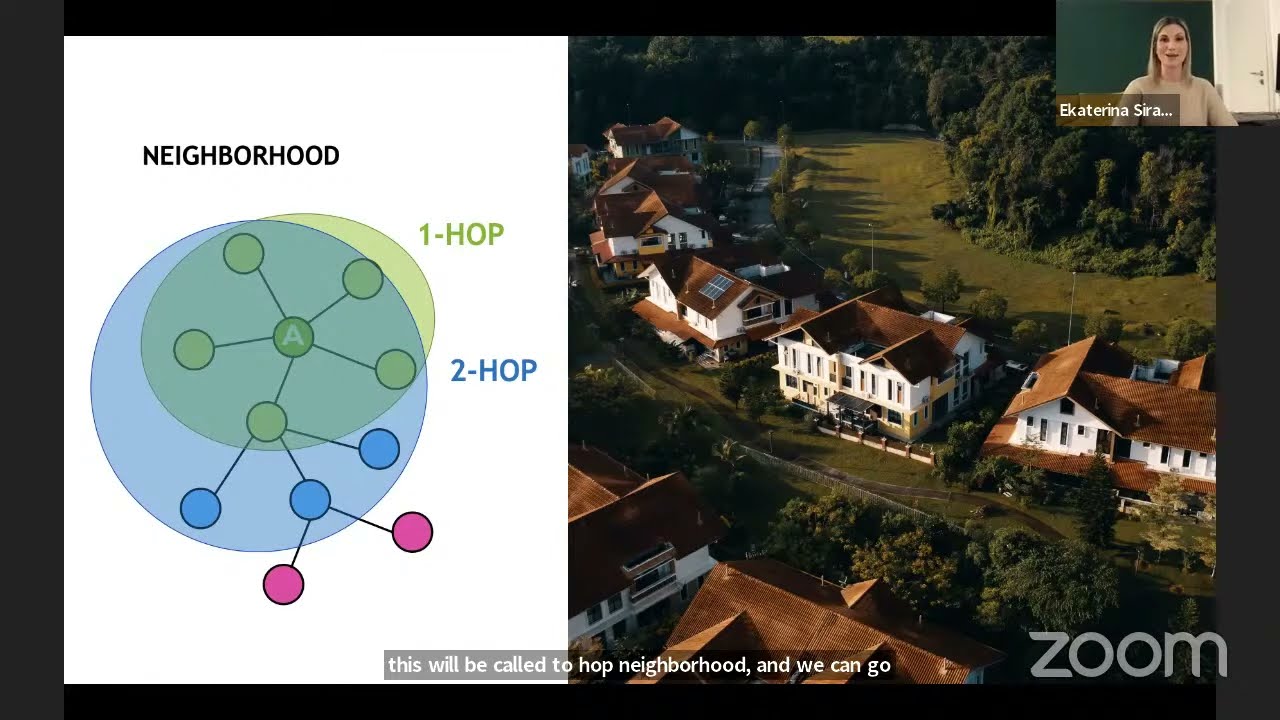
[00:17:37]First, ego-network of a given node is simply a network that is induced by the no- node itself and its neighbors.

[00:17:44]So it's basically degree 1 neighborhood network around a given node.

[00:17:49]And then what I mean by counts triangles?

[00:17:52]I mean that now, if I have this ego-network of a node, I can count how many triples of nodes are connected.

[00:17:58]And in this particular, uh, use case where, um, um, uh, the clustering coefficient of this node is 0.5, it means that I find three triangles, um, in the network, uh, neighborhood, in the, um, ego-network of my node of interest.

[00:18:15]So this means that clustering coefficient is really counting these triangles, which in social networks are very important because in social networks, a friend of my friend is also a friend with me.

[00:18:26]So social networks naturally evolve by triangle closing where basically, the intuition is if somebody has two friends in common, then more or la- uh, sooner or later these two friends will be introduced by this node v and there will be a link, uh, forming- Here, so social networks tend to have a lot of triangles syndrome and, uh, clustering coefficient is a very important metric.

[00:18:49]So now with this, the question is, could we generalize this notion of triangle accounting, uh, to more interesting structures and- and count, uh, the number of pre-specified graphs in the neighborhood of a given node.

[00:19:04]And this is exactly what the concept of graphlet, uh, captures.

[00:19:09]So the last, um, uh, way to characterize the structure of the net, uh, of the network around the given node will be through this concept of graphlets that render them just to- to- to count triangles.

[00:19:24]Also, counts other types of structures, uh, around the node.

[00:19:28]So let me define that.

[00:19:29]So graphlet is a rooted connected non isomorphic, um, subgraph.

[00:19:35]So what do I mean by this?

[00:19:37]For example, here are all, um, possible graphlets, um, that- that have, um, uh, um, different number, uh, of nodes which start with, uh, a graphlet on two nodes.

[00:19:49]So it's basically nodes connected by an edge.

[00:19:51]There are, uh, three possible graphlets on three nodes and, uh, there is, uh, and then here are the graphlets of 4-nodes.

[00:20:00]And these are the graphlets on, uh, five nodes.

[00:20:03]So now let me explain what we are looking at.

[00:20:05]So for example, if you look at the graphlets on three nodes, it is either, uh, a chain on three, um, nodes, audits or triangle, right?

[00:20:13]Its all three nodes are connected.

[00:20:15]These are all possible connected graphs on three nodes.

[00:20:19]Now why do I say there are, uh, uh, three graphlets not two?

[00:20:23]Uh, the reason for that, is that the position of the node of interest also matters.

[00:20:29]So here, for example, you can be at this position.

[00:20:32]And then the question is in how many graphs like this do you participate in.

[00:20:36]Or you can be at this other, uh, position here- position number two, and it's basically saying, how many pairs of friends do you have?

[00:20:44]And then this- this, in the case of a triangle, all this position are isomorphic, they're equivalent, so there is, uh, only one of them, so this is the, uh, position in which you may- you can be.

[00:20:55]Now, similarly, if you look at now at, uh, four node graphlets, there is, uh, um, many more of them, right?

[00:21:01]Um, uh, they- they look the following, right?

[00:21:04]You again have a chain on four nodes and you have two positions on the chain.

[00:21:07]You are either in the edge or you are one- one away from the edge- from- if you go from the other end, it is just symmetric.

[00:21:13]Here in the second, this kind of star graphlet you can either be, um, the satellite on the edge of the star or you can be the center on- of the star in a- in a square.

[00:21:22]All the positions are isomorphic, so you can be just part of the square.

[00:21:26]Here's another interesting, um, example where, um, you test three different positions.

[00:21:32]You can be- you can be here- you can be here, or you can be at position 10, which is i-isomorphic to the- to the other side in this kind of square, v dot diagonal, again, you have, uh, two different positions.

[00:21:43]And in this last fully connected graph on four nodes, uh, all nodes are equivalent.

[00:21:47]So there is- all- all positions are equivalent, so there is only one.

[00:21:50]So what this shows is that, um, if you say how many graphlets are there on five nodes, uh, there is, uh, 73 of them, right?

[00:21:57]Labeled from one, uh, all the way to 73 because it's different graphs as well as, uh, positions in these graphs.

[00:22:05]So now that we know what the graphlets are, we can define what is called Graphlet Degree Vector, which is basically a graphlet-base, uh, based features, uh, for nodes.

[00:22:16]And graphlet degree counts, um, the number of times a given graphlet appears, uh, uh, rooted at that given node.

[00:22:25]So the way you can think of this is, degree counts, the number of edges that the node touches, uh, clustering coefficient counts the number of triangles that are node touches or participates in and, uh, graphlet degree vector counts the number of graphlets that- that a node, uh, participates in.

[00:22:44]So to give you an example, um, uh, a Graphlet Degree Vector is then simply a count vector of graphlets rooted at that given node.

[00:22:54]So to, uh, to give an example, consider this particular graph here, and we are interested in the node v. Then here is a set of graphlets on two and three nodes.

[00:23:04]This is our universe of graphlets.

[00:23:06]We are only look- going to look at the graphlets all the way up to size of three nodes and node v there.

[00:23:11]Um, and then, uh, you know, what are the- what are now the graphlets instances, for example, the- the graphlets of type a, these node v participates in two of them, right?

[00:23:21]It's- one is here and the other one is there, right?

[00:23:23]So this means this one and that one.

[00:23:25]Then the graphlet of type b node v participates in one of them, right?

[00:23:30]This is, um, this is the graphlet here, right, uh, b.

[00:23:34]And then you say, how about how many graphlets of type d does, uh, node, um, sorry, of type c, does node, uh, v participate in.

[00:23:43]And it doesn't participate in any because, uh, here it is, but these two nodes are also connected.

[00:23:49]So, um, because graphlets are induced, this edge appears here as well.

[00:23:55]So for d we get zero, sorry, for c we get zero.

[00:23:58]How about for d?

[00:24:00]D is a path of- on two nodes.

[00:24:02]If you look at it, there are two instances of d. Uh, here is one and here is the other as, uh, illustrated here.

[00:24:09]So graphlet, uh, degree vector for node v would be two, one, zero, two.

[00:24:16]So two, one, zero, two.

[00:24:19]And this now characterizes the local neighborhood structure, uh, around the given node of interest based on the frequencies of these graphlets that, uh, the node v, uh, participates in.

[00:24:33]So, um, if we consider graphlets from, uh, two to five no- nodes, we can now describe every node in the network with a vector that has 73 dimensions or 73- 73 coordinates.

[00:24:48]Uh, and this is essentially a signature of a node that describes the topology, uh, of nodes, uh, neighborhood.

[00:24:54]Uh, and it captures its interact- interconnections, um, all the way up to the distance of four- four hops, right?

[00:25:01]Because, um, uh, a chain of four edges has five nodes, so if you are at the edge of the chain, which means you count how many paths of length four- do, uh, uh, lead out of that node.

[00:25:13]So it characterizes the network up to the distance, uh, of four.

[00:25:17]And, uh, Graphlet Degree Vector provides a measure of nodes, local network topology and comparing vectors now of- of two nodes, proves, uh, provides a more detailed measure of local topological similarity.

[00:25:30]Then for example, just looking at node degree or clustering coefficient.

[00:25:34]So this gives me a really fine-grained way to compare the neighborhoods, uh, the structure of neighborhoods, uh, of two different nodes, uh, in perhaps through different, uh, networks.

[00:25:44]So to conclude, uh, so far, we have introduced different ways to obtain node features.

[00:25:50]Uh, and they can be categorized based on importance features like node degree and different centrality measures, as well as structure-based features where again, no degrees like the simplest one, then, uh, that counts edges, clustering, counts triangles.

[00:26:05]And the Graphlet Degree Vector is a generalization that counts, uh, other types of structures that a given node of interest, uh, participates in.

[00:26:15]So to summarize, the importance based features capture the importance of a node in a graph.

[00:26:21]We talked about degree centrality, um, and we talked about different notions of, uh, centrality closeness, betweenness, um, as well as, um, the eigenvector, uh centrality.

[00:26:34]And these types of features are using in predicting, for example, how important or influential are nodes in the graph.

[00:26:40]So for example, identifying celebrity users in social networks would be one, uh, such, uh, example.

[00:26:47]Um, the other type of node level features that we talked about, were structured based-fea- structure-based features that capture the topological properties of local neighborhood around the node.

[00:26:59]We talked about node degree, clustering coefficient and graphlet degree vector and these types of features that are very useful, uh, for predicting a particular nodes role, uh, in the network.

[00:27:10]So for example, if you think about predicting protein function, then, um, these type of graphlet, uh, features are very useful because they characterize, uh, the structure of the, uh, network, uh, around, given, uh, node.