TFT Forecasting: Energy Demand & Deep Learning
Learning Goal: Implement and evaluate deep learning-based multivariate time series forecasting models using Temporal Fusion Transformers for energy grid demand prediction.
- Prerequisites: Basic understanding of algebra and programming concepts. No prior machine learning experience required.
- Estimated Total Study Time: 38 Hours
Module 1: Programming & Data Science Foundations
To build advanced deep learning systems, you must first master the fundamental tools of data science. This module establishes a solid foundation in Python, comprehensive data manipulation with Pandas (focusing heavily on temporal indices and datetime mechanics), and the core statistical principles required to interpret real-world datasets.
Recommended Videos

Why this video is valuable: This introductory video provides a robust high-level map of the data science lifecycle. It establishes the critical baseline of why Python is preferred in scientific computing and introduces the initial packages you will rely on throughout this curriculum.

Why this video is valuable: Data cleaning and transformation are 80% of any deep learning project. This intensive tutorial quickly moves you from zero to a functional understanding of Series and DataFrames, showing you how to ingest, filter, and restructure tabular data.

Why this video is valuable: Time-series forecasting depends entirely on precise temporal indexing. This video is an essential deep dive into converting raw strings to Pandas datetime objects, extracting time-based features (hour, day of week, month), and utilizing date-anchored indexes for seamless slicing.

Why this video is valuable: You cannot evaluate forecast errors or feature correlations without statistical foundations. This comprehensive lecture explains central tendency, variance, dispersion, and distributions—mathematical prerequisites for understanding signal vs. noise in multivariate systems.
Knowledge Checkpoint
- Install a Python virtual environment and set up a Jupyter notebook interface.
- Import an arbitrary CSV, convert a date column using
pd.to_datetime(), and set it as the DataFrame index. - Create engineered temporal features like
df['hour']anddf['day_of_week']from a datetime index. - Compute mean, variance, and standard deviation manually and verify them using Pandas methods.
Module 2: Introduction to Machine Learning & Time Series
With programming fundamentals secured, you are ready to transition to modeling. This module introduces the core paradigms of machine learning, guides you through implementing classical statistical time series models (like ARIMA), and teaches you how to rigorously evaluate forecasting accuracy using standard metric formulations.
Recommended Videos

Why this video is valuable: This introductory video frames the central paradigm shift of machine learning: moving from explicit step-by-step programming to learning underlying representations and statistical patterns directly from raw input-output pairs.
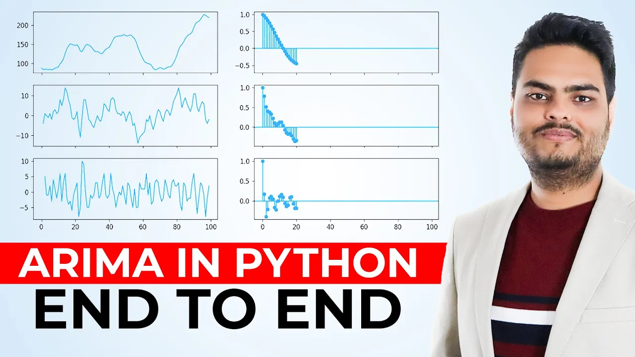
Why this video is valuable: Before jumping to deep learning, you must establish a baseline. This practical video shows you how to test for stationarity, determine lag parameters, fit an AutoRegressive Integrated Moving Average (ARIMA) model, and output out-of-sample statistical predictions.

Why this video is valuable: You cannot optimize a model you cannot measure. This clear math tutorial explains the formulation, calculation, and practical interpretation of MAE, MSE, RMSE, and MAPE, showing how outliers influence each error calculation.
Knowledge Checkpoint
- Differentiate between supervised learning, unsupervised learning, and classic time-series forecasting.
- Explain the necessity of stationarity in ARIMA models and how differencing achieves it.
- Programmatically split a time series dataset sequentially (retaining temporal order) instead of using a randomized train-test split.
- Calculate Root Mean Squared Error (RMSE) and Mean Absolute Error (MAE) mathematically on a set of actual vs. predicted values.
Module 3: Deep Learning & Sequential Models
Classic statistical models fail when temporal relationships are highly non-linear or multivariate. This module introduces the core mechanics of Artificial Neural Networks, transitions into Recurrent Neural Networks (RNNs) and Long Short-Term Memory (LSTM) cells, and teaches you how to construct these models from scratch using PyTorch.
Recommended Videos

Why this video is valuable: Widely recognized as one of the best visual introductions to deep learning, this video deconstructs neural network layers, weights, biases, and activation functions, helping you visualize how complex vector mathematics transforms inputs into outputs.

Why this video is valuable: Standard feed-forward neural networks struggle with temporal data because they lack persistence over time. This video provides a detailed structural breakdown of LSTMs, explaining how the cell state, forget gate, input gate, and output gate prevent vanishing gradients over long horizons.

Why this video is valuable:
This tutorial bridges the gap between LSTM theory and clean PyTorch code. You will learn how to structure multidimensional arrays, define an LSTM architecture subclassing torch.nn.Module, and run a multi-step training loop on sequential target data.
Knowledge Checkpoint
- Draw a diagram of a standard neural network node showing input summation, bias addition, and activation function execution.
- Explain the vanishing gradient problem in standard Recurrent Neural Networks and identify which LSTM component mitigates this.
- Implement a custom PyTorch dataset class that converts a sliding window of historical time steps into an input tensor
(batch_size, seq_len, features). - Code a simple forward pass of an LSTM using PyTorch's
nn.LSTMand check the shapes of the output and hidden state tensors.
Module 4: Attention Mechanisms & Transformer Networks
While LSTMs process inputs step-by-step, the Transformer architecture revolutionized sequence modeling by processing entire sequences at once. This module breaks down the Self-Attention mechanism, Positional Encodings, and multi-headed Transformer architectures that form the backbone of modern forecasting.
Recommended Videos

Why this video is valuable: This conceptual video explains the core intuition behind attention. You will see how a model calculates context-dependent weights, allowing it to focus on relevant historical steps rather than weighing all past observations equally.

Why this video is valuable: This video breaks down the mathematical operations of Self-Attention. It clarifies how Query (Q), Key (K), and Value (V) matrices are generated, and how their dot-product attention maps determine temporal relationships.
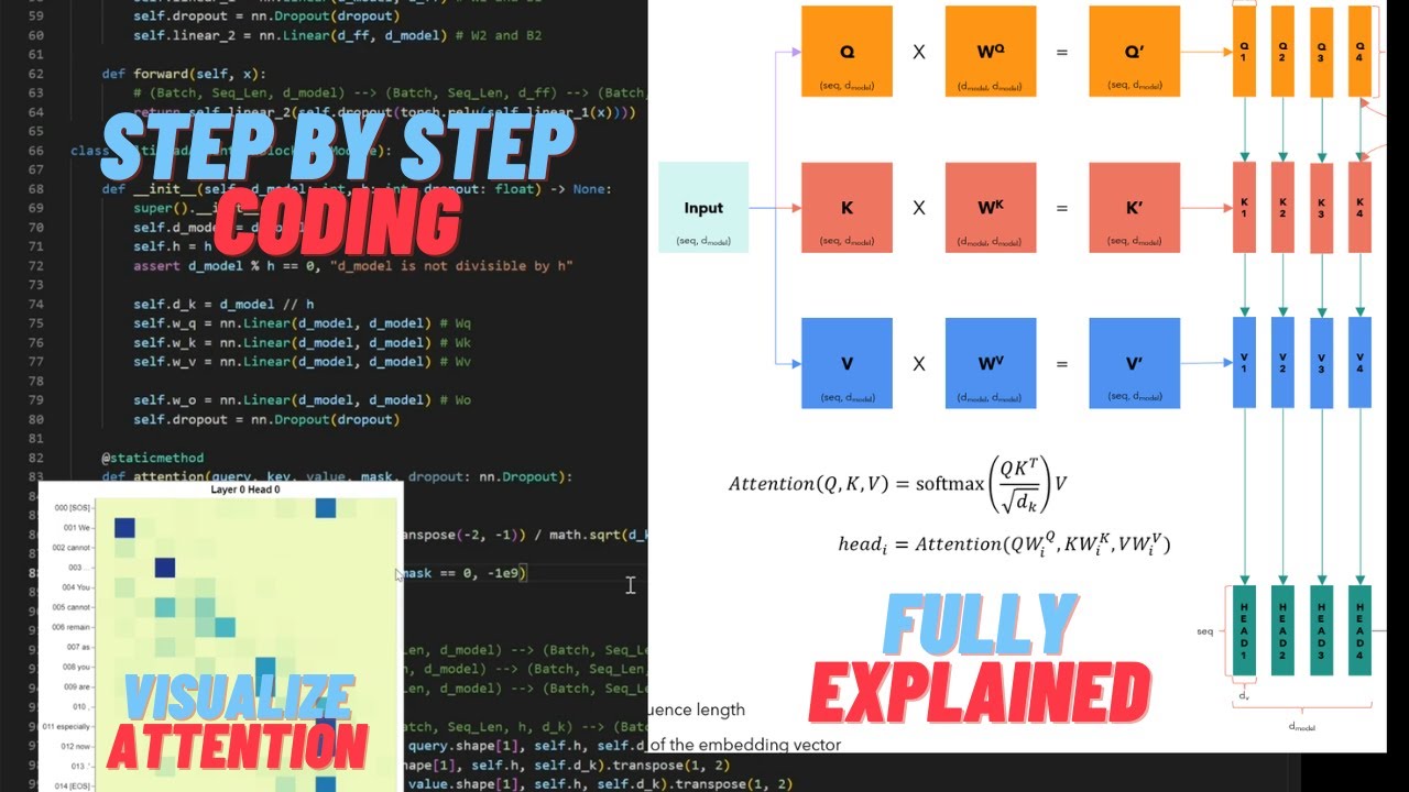
Why this video is valuable: The ultimate test of understanding is implementation. This masterclass walks through every line of code needed to write a complete Transformer from scratch in PyTorch. It provides deep technical insights into scaled dot-product attention, multi-head configurations, and layer normalization.
Knowledge Checkpoint
- Explain the mathematical formula for Scaled Dot-Product Attention: .
- Explain why Positional Encodings are necessary for Transformers but not for LSTMs.
- Explain how Multi-Head Attention allows a model to jointly attend to information from different representation subspaces at different positions.
- Write a raw PyTorch class that performs scaled dot-product attention on three input tensors: Queries, Keys, and Values.
Module 5: Deep Dive into Temporal Fusion Transformers (TFT)
Now we focus on the specialized model for time series forecasting: the Temporal Fusion Transformer (TFT). This module deconstructs the TFT architecture, examining how it handles static metadata, known future inputs (like weather forecasts), and historical target variables, while maintaining full feature interpretability.
Recommended Videos

Why this video is valuable: This video explains the practical benefits of the TFT architecture over standard Transformers. It details how the model manages different types of inputs (static metadata, known future inputs, and unknown historical targets) and outputs multi-quantile probabilistic forecasts.
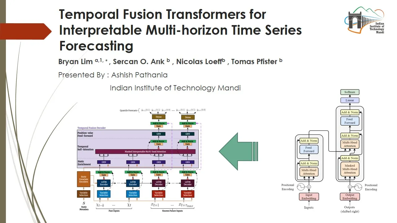
Why this video is valuable: This video walks through the academic paper behind TFT. It breaks down the internal architecture, explaining how the Variable Selection Networks filter out irrelevant inputs and how the temporal self-attention layer tracks long-term patterns.

Why this video is valuable: This short video highlights why TFT is particularly well-suited for complex real-world forecasting tasks, emphasizing its capability to naturally incorporate static, past, and future covariates.
Key Architectural Deep Dive
While the videos provide a strong conceptual overview, implementing TFT requires understanding its specialized internal modules:
        +---------------------------------------+
        |      Multi-Quantile Outputs           |
        +---------------------------------------+
                            ^
        +---------------------------------------+
        |  Temporal Self-Attention Layer        | (Processes temporal dynamics)
        +---------------------------------------+
                            ^
        +---------------------------------------+
        |  Variable Selection Networks (VSN)    | (Weights static/dynamic inputs)
        +---------------------------------------+
                            ^
        +---------------------------------------+
        |  Gated Residual Networks (GRN)        | (Allows adaptive model capacity)
        +---------------------------------------+
           /                |                \
+------------------+ +-------------+ +------------------+
| Static Covariates| | Known Future| | Unknown Past/Tgt |
+------------------+ +-------------+ +------------------+
- Gated Residual Network (GRN): This component allows the model to adaptively skip unused parts of the network. If a simple linear relationship is sufficient for a specific feature, the GRN can bypass non-linear transformations using its gating mechanism, preventing overfitting.
- Variable Selection Network (VSN): Time series often contain noisy, irrelevant features. The VSN calculates attention weights for each input variable at each step, allowing the model to ignore noisy inputs and focus on key drivers.
- Temporal Self-Attention: This layer processes temporal relationships across time steps, allowing the model to capture cyclic patterns (like daily or seasonal energy demand) over long horizons.
Knowledge Checkpoint
- Categorize the following features into Static, Known Future, or Unknown Past covariates for energy forecasting: calendar day, historical demand, station ID, predicted wind speed.
- Explain how Gated Residual Networks (GRN) allow the TFT architecture to adaptively scale down to simple linear models if complex non-linear structures are unnecessary.
- Explain how the Variable Selection Network (VSN) calculates feature importance to provide model interpretability.
- Explain why forecasting in quantiles (e.g., 10th, 50th, 90th percentiles) is more valuable for risk management than a single point prediction.
Module 6: Energy Grid Demand Project Implementation
Now you will apply what you have learned to a practical, end-to-end energy forecasting project. Using real-world datasets, you will prepare inputs, define the forecasting model, and train a multivariate predictor.
Technical Note: Dedicated video coverage for the niche
pytorch-forecastingpackage is limited. This module provides a complete blueprint for organizing covariates, defining the training dataset, and setting up the API calls for a Temporal Fusion Transformer model.
Recommended Videos

Why this video is valuable: This practical walkthrough demonstrates how to implement a TFT model using Python-centric forecasting libraries (such as Darts), showing you how to ingest data, configure hyperparameters, and evaluate model performance.

Why this video is valuable: This start-to-end project overview shows how to handle electricity datasets, clean raw demand observations, engineer holiday variables, and structure a complete machine learning training pipeline.

Why this video is valuable: This video provides a practical reference for constructing custom PyTorch Dataset classes for sequence data. It explains the mechanics of using historical lookbacks and forecast horizons to map multidimensional inputs into clean batch tensors.
Implementation Blueprint: Dataset Preparation & TFT Setup
To implement a TFT model on energy demand data using modern deep learning frameworks, you must structure your variables into distinct groups. Below is the blueprint for mapping your dataset to the TimeSeriesDataSet interface in PyTorch Forecasting:
from pytorch_forecasting import TimeSeriesDataSet from pytorch_forecasting.metrics import QuantileLoss
1. Define feature classifications based on temporal characteristics
static_categoricals = ["station_id"] # Non-changing metadata (e.g., location ID) time_varying_known_reals = [ # Features known ahead of time "hour", "day_of_week", "month", # Time identifiers "predicted_temperature", # Numerical forecasts ] time_varying_unknown_reals = [ # Target variable and historical measurements "energy_demand_kw", # The historical target to forecast "observed_wind_speed", # Only known up to the present moment ]
2. Instantiate the TimeSeriesDataSet
training_dataset = TimeSeriesDataSet( data=df_train, time_idx="time_step_index", # Integer index incrementing by 1 per step target="energy_demand_kw", # Target variable group_ids=["station_id"], # Entity identifier max_encoder_length=168, # Lookback window (e.g., 7 days of hourly data) max_decoder_length=24, # Forecast horizon (predict 24 hours ahead) static_categoricals=static_categoricals, time_varying_known_reals=time_varying_known_reals, time_varying_unknown_reals=time_varying_unknown_reals, target_normalizer=None, # Use default or scaling of choice )
This structural blueprint maps variables to the TFT architecture, ensuring that future lookaheads are only performed on variables classified as "known reals."
Knowledge Checkpoint
- Prepare an energy load dataset with an integer index and continuous time steps.
- Define the lookback window (encoder length) and forecasting horizon (decoder length) based on your project requirements.
- Map all features to their correct classifications (
static_categoricals,time_varying_known_reals,time_varying_unknown_reals). - Configure a Quantile Loss function to predict the 10th, 50th, and 90th percentiles of energy demand.
Course Map
This map outlines the recommended learning order and module dependencies:
Key People Index
Notable researchers, educators, and institutions mentioned across this curriculum:
- Bryan Lim: Lead author of the foundational research paper Temporal Fusion Transformers for Interpretable Multi-horizon Time Series Forecasting.
- Grant Sanderson: Creator of the channel 3Blue1Brown, renowned for visually intuitive explanations of neural network mathematics, gradient descent, and backpropagation.
- Ashish Vaswani: Lead author of the seminal paper Attention Is All You Need, which introduced the Transformer architecture to deep learning.
- Drew Kaul: Stanford researcher and Deep Learning instructor who specializes in translating complex theoretical frameworks into practical PyTorch codebases.
Final Self-Assessment
Test your understanding of the complete curriculum by completing the following checklist:
- Explain the differences between static categoricals, time-varying known reals, and time-varying unknown reals in the context of the TFT architecture.
- Programmatically convert raw energy datasets into three-dimensional PyTorch tensors with shapes of
(batch_size, sequence_length, features). - Explain how Gated Residual Networks (GRNs) allow a model to dynamically control its complexity and prevent overfitting on smaller datasets.
- Explain how the Variable Selection Network (VSN) computes feature importance to make predictions interpretable.
- Calculate standard forecast accuracy metrics (MAE, RMSE, MAPE) on a set of validation predictions.
- Explain why traditional cross-validation (like random k-fold splits) fails on time series data, and how to use sequential temporal validation instead.
- Set up a multi-quantile loss function to compute probabilistic forecasts (predicting range intervals instead of single points).
- Successfully train, validate, and evaluate an interpretable Temporal Fusion Transformer on multivariate energy grid data.