![[TUTORIAL] PYTHON para Análise de Dados - Aprenda do ZERO](https://i.ytimg.com/vi/FZODEbfcDwU/maxresdefault.jpg)


![Как анализировать данные с Python библиотеками Pandas и Numpy [GeekBrains]](https://i.ytimg.com/vi_webp/lLf6Qt6wSJ8/maxresdefault.webp)






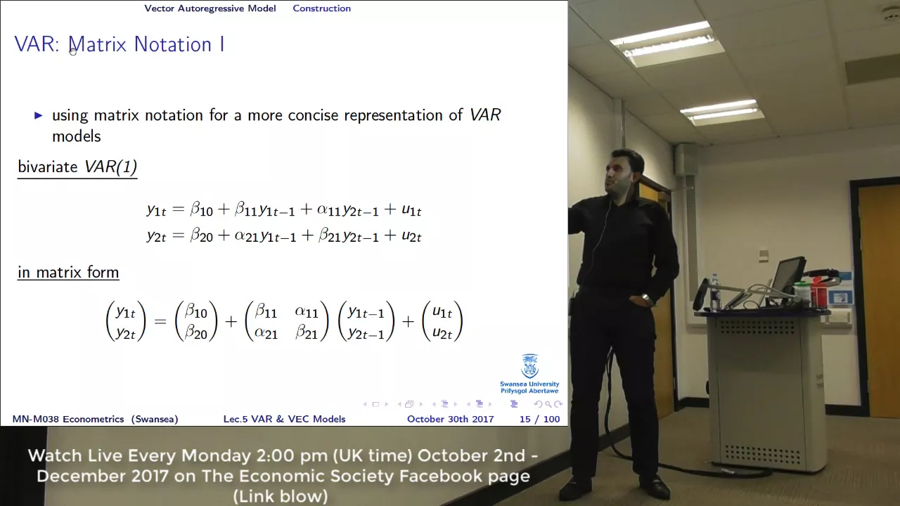
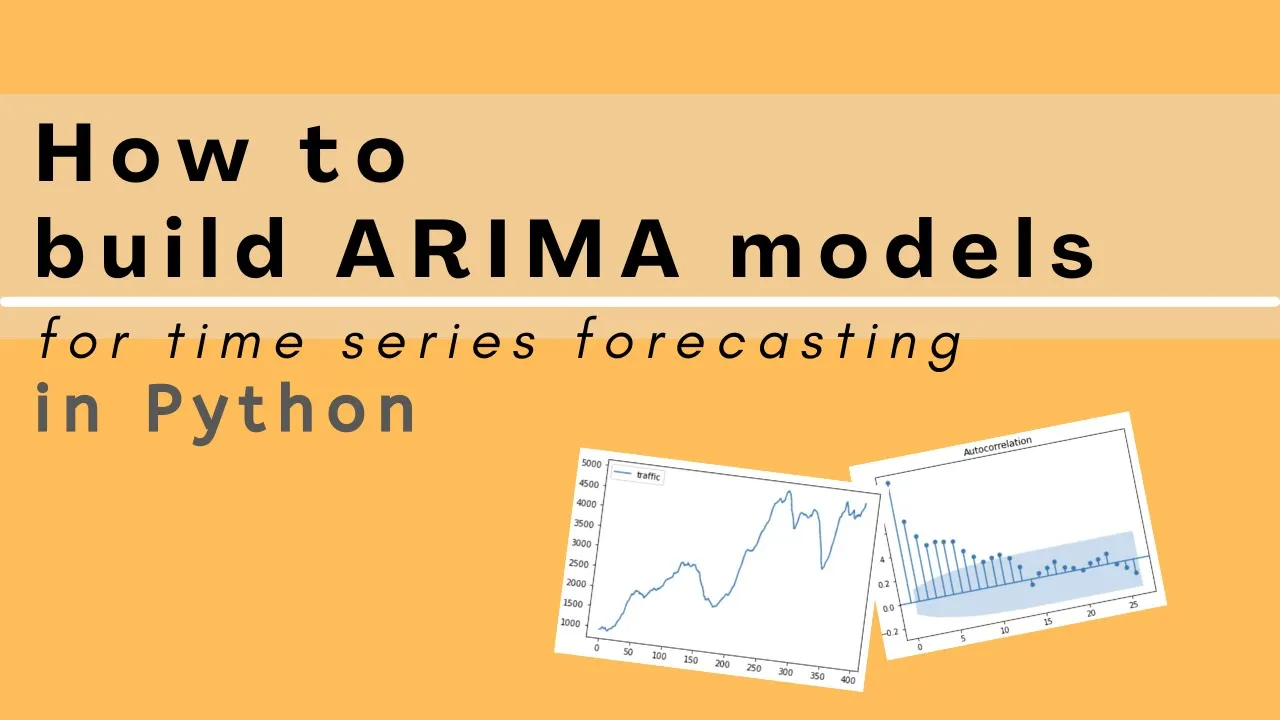





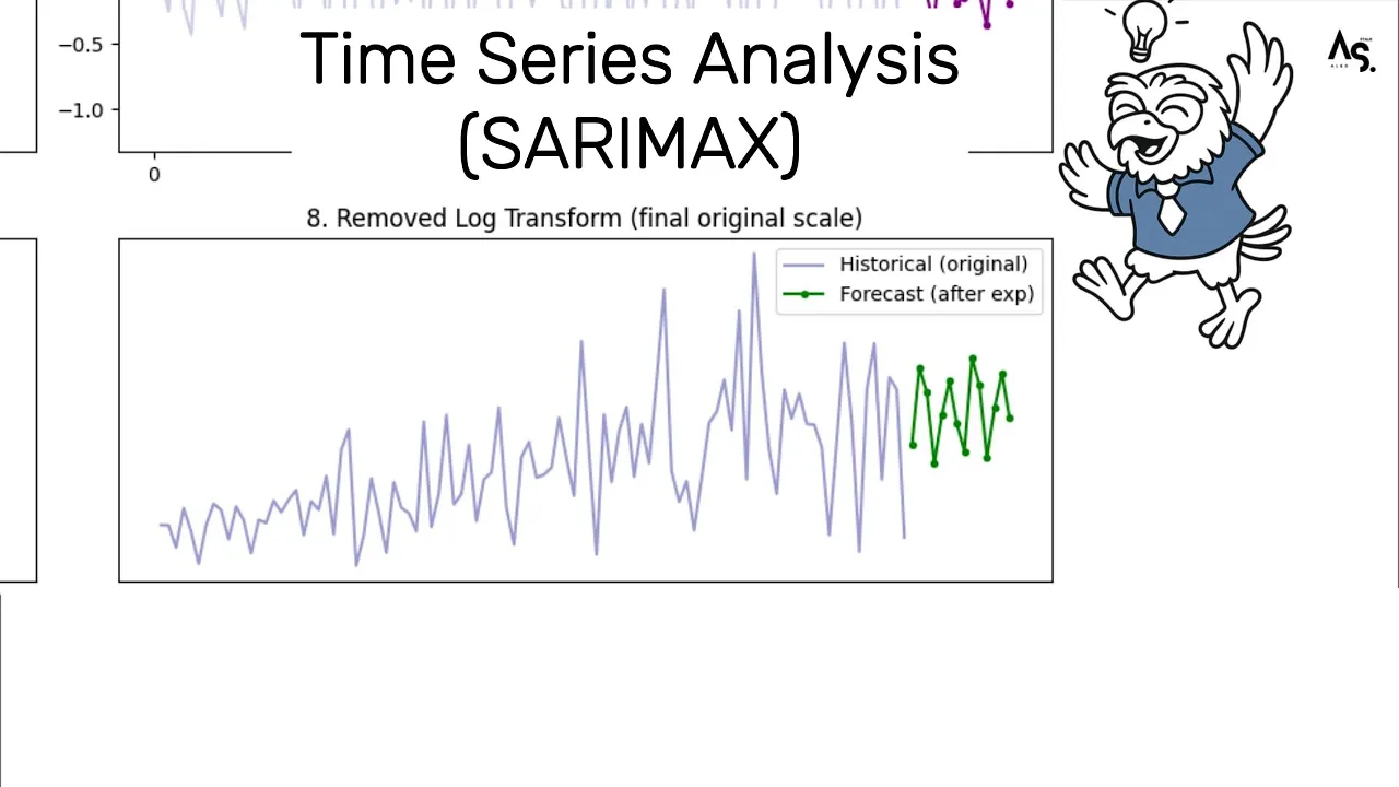








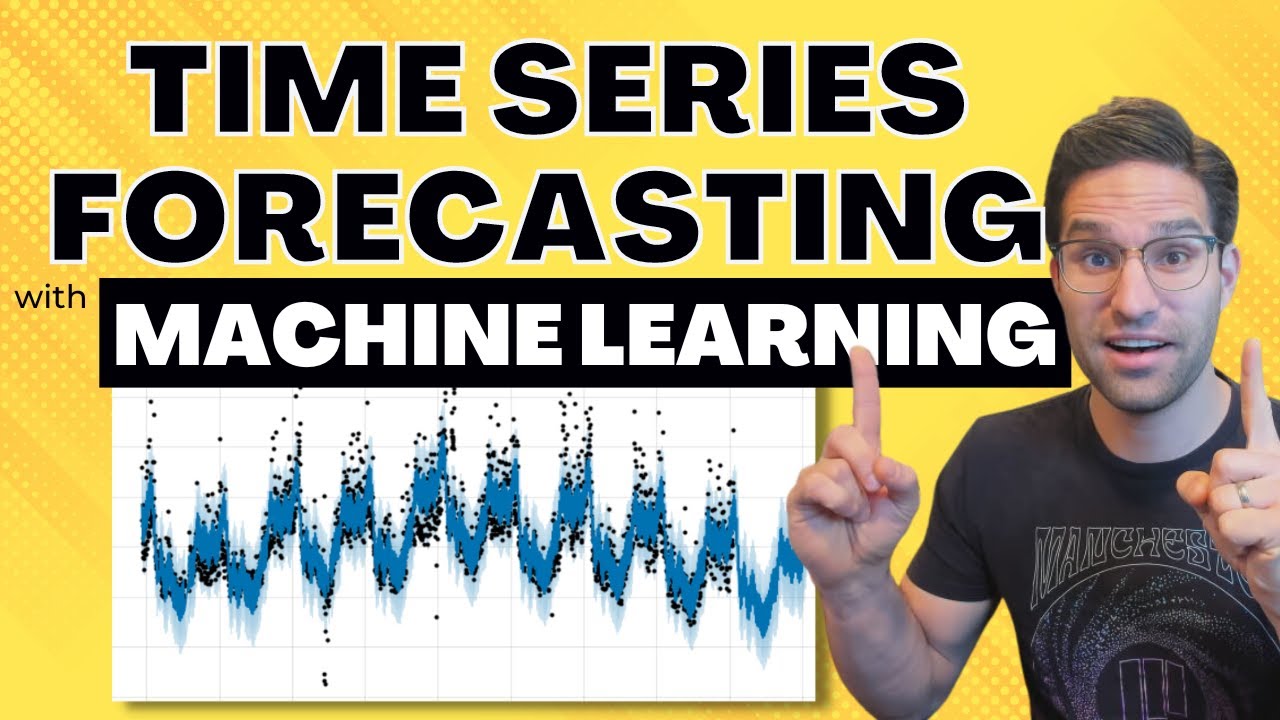
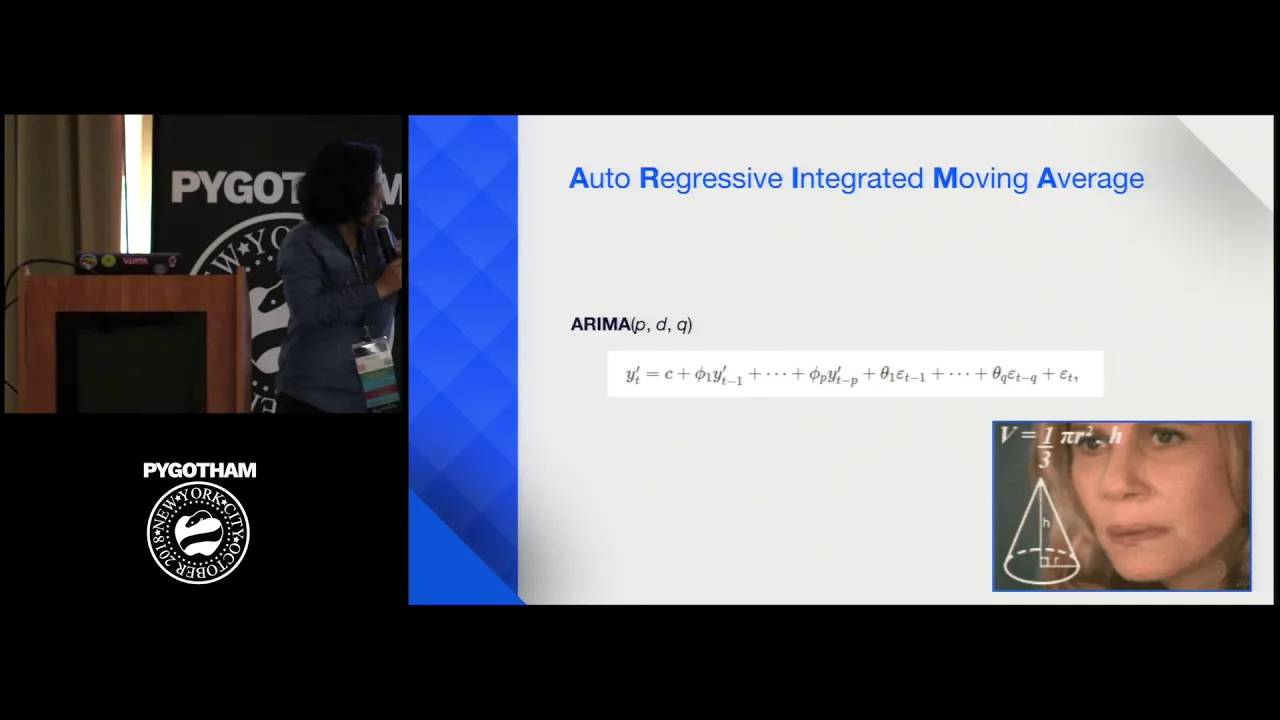

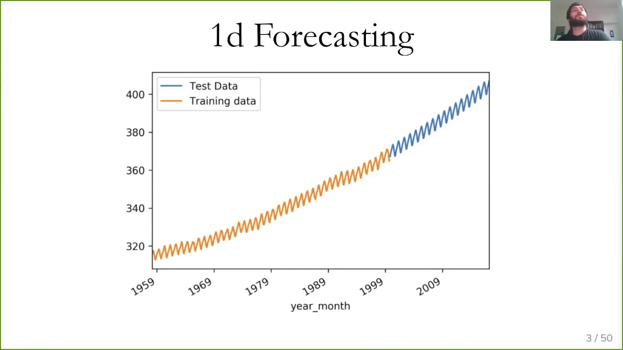
This video demonstrates an end-to-end implementation of ARIMA (Auto Regressive Integrated Moving Average) for time series forecasting in Python, covering key steps including data import and cleaning, stationarity checks using rolling statistics and ADF test, log transformation and differencing to achieve stationarity, determining AR and MA orders using ACF and PACF plots, fitting the ARIMA model, and transforming predictions back to original scale; the tutorial also introduces auto ARIMA for automated parameter optimization.
Time Series Forecasting in Python: Implementing ARIMA Models End-to-End
Added:Basic Python programming proficiency, including familiarity with data manipulation libraries like Pandas and NumPy.
Fundamental concepts of time series analysis, such as identifying trend, seasonality, and noise components.
Basic understanding of statistical stationarity and why non-stationary data poses challenges for forecasting.
Familiarity with Autocorrelation (ACF) and Partial Autocorrelation (PACF) functions used to identify correlation in lagged data.
Expanding to SARIMA and SARIMAX models to incorporate seasonal patterns and external exogenous variables.
Implementing advanced time series validation techniques, such as rolling-window (walk-forward) cross-validation.
Exploring volatility and heteroskedasticity in financial data using ARCH and GARCH models.
Transitioning to machine learning and deep learning approaches for forecasting, such as Prophet, XGBoost, and Long Short-Term Memory (LSTM) networks.
53.7K views1.1Klikes16:28Original Release: 2020-12-16
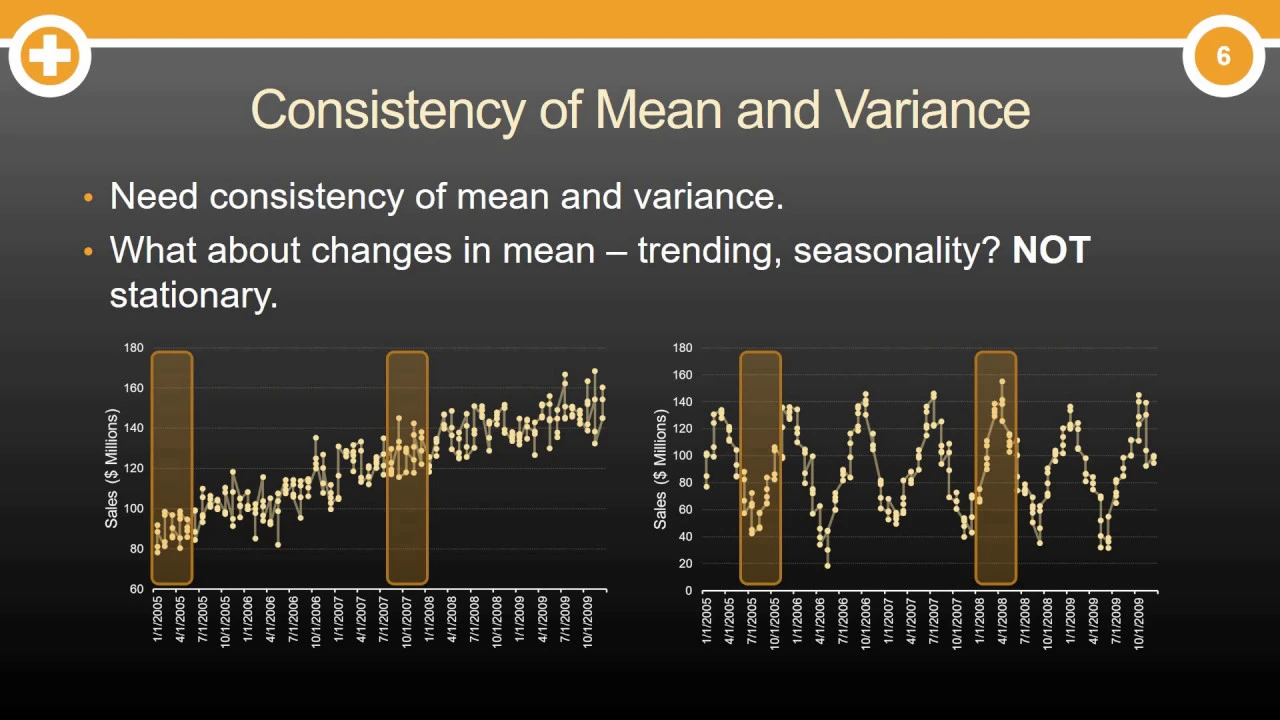
hey guys welcome to unfold data science this is aman here and i am a data scientist as you can see on your screen guys today i am going to show you an end-to-end implementation of time series basically using the arima method so most of you would be heard would have heard about the method arima which stands for auto regression integrated moving average or auto regressive integrated moving average right so there are three components of arima one is ar next is i and this is m a r stands for auto regression m a for moving average and i for differencing term i have already explained ar and m a in my in the same playlist in my previous videos i am giving the link you can watch those videos as well but in this video we will see a end-to-end implementation of arima as a model okay so what i am doing here is i am just setting my working directory guys here as you can see this image was used in my last video as well i am importing the data cleaning doing some stationarity check i will tune i will train the model arima model then i will do some prediction and then i will tune the model we will do all this step by step this video might get a little longer but i request you to watch till end so that you get a overall understanding of how to fit a time series model so first thing is guys importing data okay so wherefrom i have taken data i have taken data from this place okay so a credit to kaggle and in kaggle credit to mr bhupani who has uploaded this data so this data gives you stock market data basically the nifty data for different different stocks okay so you can download the data from here i'll give you the link and i can give you the data as well okay in this data i am taking one particular company hcl tech okay so hcl is a software company hcl tech data i'm taking and i'm just printing the first 30 records of hcl tech data so as you can see guys the on from the year 2000 okay symbol hcl tech hcl tech is the name of the company previous close this is the stock market price open high low last all these things right what was the previous close what was the day high what was the day low all these information of this stock price right so we will be using this previous close column as our main column for on what target or on what number this stock price will close for that particular day okay so going forward i will use this column only so what i am doing here is i am dropping all the any columns so that our analysis is not disturbed i have many records so i can drop some of these ns right next thing very important thing guys you have to necessarily make a index column in any of your time series analysis so as you can see there is one column called date this date column i am making it as the index column for this analysis okay so i'm saying hcl take stock data dot index is equal to pd dot date time this date so it will take this date as my date column okay now i am taking as i told you i'll be using only one column and i am taking the data from 2013 as a year okay 2013 from january to december as you can see here right now if you come down guys so i'm just printing a describe of my data so nearly one year of data you will see some 230 uh entries the reason for that is on saturday and sunday stock market holiday is there and some more holidays right so nearly 230 entries the mean is 852 and other percentiles you can see here now let us plot this data and see how it is looking like okay so this is the plot of the hcl tech stock data guys for 2013 entire year okay this is first month 2013 this is 11th month and then the 12th month okay now as you can see i have knowingly taken this data the reason being it is showing some kind of i can say it's not an easy time series okay so there is no clear-cut trend sometime it goes up sometimes it comes down again it comes down goes up comes down so there's no fixed what you say seasonality component or trend is there upward trend is there but seasonal components we cannot see clearly in this image okay so how do we see the next thing about these time series the very first thing is we should know whether this is a stationary time series how do you see whether the time series is stationary or not again i have created a video on that you can watch that video to keep it simple you can use two methods one is using rolling statistics which means rolling mean as standard deviation next is using the key fuller test both these methods i have shown you in this video the link is right here you must watch this video as well okay and then what i'm trying to do here is i'm trying to create some rolling statistics if you see rolling mean is equal to hcl stock data dot rolling 12 mean which means i am taking a rolling mean of last i'm taking a rolling mean of 12 entries okay similarly rolling stat standard deviation of 12 entries and don't worry about these plot things guys this is just about plotting these two numbers okay now i am plotting the original series with the rolling okay so original is blue in color rolling mean is red in color and rolling standard deviation is black in color so as you can see rolling standard deviation is more or less constant over the time okay so what is the prerequisite for a series 2 called stationary mean should be constant over a time and standard deviation should be constant over a time now we can see rolling standard deviation is kind of constant but rolling mean is not constant which definitely means that this series is not a stationary series right now coming back to how to make this series stationary plt dot plot figure size is equal to 16 7 figure size is equal to so i am just giving the figure size and then the first thing we can do is to make series stationary is we can take a log transformation of the series or we can take many transformations so here i am taking a log transformation you can take a square root transformation cube transformation many kind of transformation we don't know what transformation will make our series stationary okay so i'm just trying with log transformation np dot log will do the log transformation of my series and i am plotting that when i plot that this time series is not becoming stationary as you can see strengthening time series will not show a trend like this right to to double sure that this time series is not stationary we will just decompose it into seasonal components okay how to do that from stats model tsa or seasonal import seasonal decompose decomposition is equal to ts log and what this will do is it will give you the different components of your time series whether it is a seasonal trend okay so if you see this chart here that that particular time series has been broken into four components the first one is the original series second one is the trend component of that particular series third one is the seasonality component of that particular series and fourth one is the residual component of that particular series so it is very evident from here that trend component is contributing more to the original time series right now we know series is not stationary even after log transformation as well so i will do something else what is that something else so i will create a difference to time series what is difference to time series i will shift the time series by 1 and subtract from the original time series that is what i am doing here guys ts log difference means the log time series and then i get the difference is equal to ts log minus ts log shift 1 so i will get a differenced time series as a result of this and then i expect this difference time series to be stationary at least okay so same way i am plotting the rolling mean and rolling standard deviation on this time series now okay to check whether this is a stationary or not when i do that guys you can see the blue one is my difference to time series okay the black one is my rolling standard deviation and the red one is my rolling mean now you can see there is no upward pattern in the mean and there is no upward pattern in the standard deviation so by the definition of stationarity if i take mean between these two points and if i take mean between these two points then there will not be too much of difference between these so i assume this time series will be a stationary time series all this hard work of taking the log and taking the difference and seeing the mean seeing the standard deviation is because we want series to be stationary otherwise our model will not fit well on the series okay and also we have to remember what all transformations we have done for example here we have done log and here we have done differencing just remember these two okay now this time series looks looks uh good guys good in the sense looks stationary if you want to cross validate you can do a decay fuller test as well okay moving on to the next steps guys now we have a time series in hand let us try running acf and pacf now what are these two things i have explained this also in one of my video in time series playlist these are important to determine what will be the order of your ar component and m a component in the arima model okay one is called autocorrelation plot second is called partial autocorrelation plot okay was the video on these topics as well link i am providing okay now what i am doing is i am plotting acf chart and psef chart for that difference to time series okay let me do that this is how your psef and acf looks like now how do you determine from first one is auto correlation second one is partial autocorrelation the important thing to understand here guys is whenever you are running a arima model you do not know what order of a r and m a or i will be good for your model okay so these charts help you understand in that now the thumb rule here is whatever the highlighted part you see here these are called confidence intervals okay and the first line that crosses this chart the first line that crosses this chart is the line of your order whatever you want now here you can see i am just considering line number two so this is point number zero point number one and point number two here point number two is not crossing the uh interval but it is just touching the tip okay so i will consider order of ar as two okay from autocorrelation order of m a also i will consider 2 from partial auto correlation okay i do not know whether that is the best fit but to start with let us go with 2 0 2 as pdq okay and d i am starting with 0 let us see what happens ok so what i am doing here from stats model arima model import arima arima give your time series okay and then order will be 2 1 and 2 okay so here i am starting with order 2 1 2 as you can see right and then when i run these guys you will see that this red one is the fitted values which means i am predicting for that model and this other one the light green one is the actual values so this is how the time series model is fitting on the data now what we need to do is we need to we have done many transformations right so we need to taking result back to the original scale so i told you we we did uh np dot log which means we did the log transformation we did some bit of differencing right so in the first step what we are doing is we are just taking the fitted values in a in a series in the second step what we are doing is we are taking the cumulative sum the reason being we differenced the time series okay and in the third one what we will do is we will take the np dot as you can see there is one step before this what we are doing is we are taking log prediction and we are adding this addition is to compensate for the differencing okay we did that differencing if you see one one values you will understand what is happening right and then in the last step if you see we are doing np dot exponential so what is the reverse of log guys exponential right so since we had done log so here we are doing exponential so np dot exponential arima log prediction and then when i run this you will see that this this pink one this light pink one sorry the orange one is your predicted value and the light blue one is your actual values here okay now there are many things about this time series which we need to understand one is this time series is very well capturing the trend component but the time series is not capturing some of these unexpected ups and downs there are some minor ups and downs in the time series but volume of those is not as far with the actual time series okay and that is where we are getting some rmse value here how to improve that now if you remember we started from pdq as 2 1 2 okay we do not know if some other pdq will give a better result for the same time series there is another way in which we can do it the way is known as auto arima before that you can predict using that same model resultary image dot predict and for whatever to whatever entry you want to predict you can give in the four so for index number 10 to index number 20 i want to predict and these are the predictions okay i was talking about auto arima as well so auto arima comes from a package called pmd arima you can take your auto arima you can give your different values of pdq and run that in a loop okay what will happen is it will give you the best pdq values for your model now when i run that auto arima for this model i got the best pdq as 0 1 0 when i plugged in 0 1 0 in my model i was not able to get a better performance so what i am suspecting is there could be a better way of making this time series stationary and there could be a better way of doing the transformations so i leave it to you you take the data you see this notebook also and you try to implement this time series in your own local environment and try to see what transformations help you what what other things you can do so that your time series performance can be better okay but all in all this was an implementation of arima all the steps involved just to reiterate you import the data you clean the unnecessary stuff you ensure data is stationary and then you take it to the model and then you decide and which which is the optimal pdq for your model you run the time series if there is performance can be improved you improve with auto arima or other differencing methods or transformation methods right so this is all in all that i wanted to show you in this video guys let me know what doubt what questions you have i'll see you all in the next video till then all of you stay safe and take care
Up Next
16:58
Regression Metrics Explained: MAE, MSE, RMSE, MAPE, MPE | Machine Learning
@professor-ryanahmed
41.7K views•2019-06-26

57:48
Secure Multiparty Computation (MPC): Foundations & Challenges
@SimonsInstitute
7.3K views•2015-05-28

13:03
Bypassing Tor Censorship: Bridges and Pluggable Transport Guide
@Coding_ForEveryone
397 views•2024-06-11

18:41
Neural Networks Explained: Math, Layers, and Learning Fundamentals
@3blue1brown
21.9M views•2017-10-05
Related Study Plans & Knowledge Roadmaps
Structured learning paths in Artificial Intelligence
artificial-intelligence
Aligning LLMs: DPO, TRL & Custom Datasets
01Foundations of Python & Machine Learning
02Transformers and Large Language Models (LLMs)
03Aligning LLMs: SFT and RLHF
+ 3 more learning modules
24h6 modules
Explore Roadmap
artificial-intelligence
Federated Learning: PyTorch, Flower & Privacy
01Python & Machine Learning Foundations
02Deep Learning Basics with PyTorch
03Introduction to Federated Learning
+ 2 more learning modules
35h5 modules
Explore Roadmap
artificial-intelligence
Securing LLMs: Guardrails AI & NeMo Gateway
01Introduction to LLMs, Python, and APIs
02Understanding LLM Vulnerabilities & Threats
03Defending LLMs with Guardrails AI
+ 2 more learning modules
15h5 modules
Explore Roadmap
artificial-intelligence
Building Recommenders: Two-Tower & Vector DBs
01Foundations of Python & Machine Learning Basics
02Introduction to Recommender Systems
03Deep Learning & Representation Learning
+ 3 more learning modules
75h6 modules
Explore Roadmap