









![MathAcademy -- Foundations II (98%) [Study with me]](https://i.ytimg.com/vi/OjBpiGQvNYA/maxresdefault.jpg)










![O Único Robô que você precisa para fazer R$10.000 por mês [Guia Completo]](https://i.ytimg.com/vi_webp/NhbnI-A2Ry8/maxresdefault.webp)

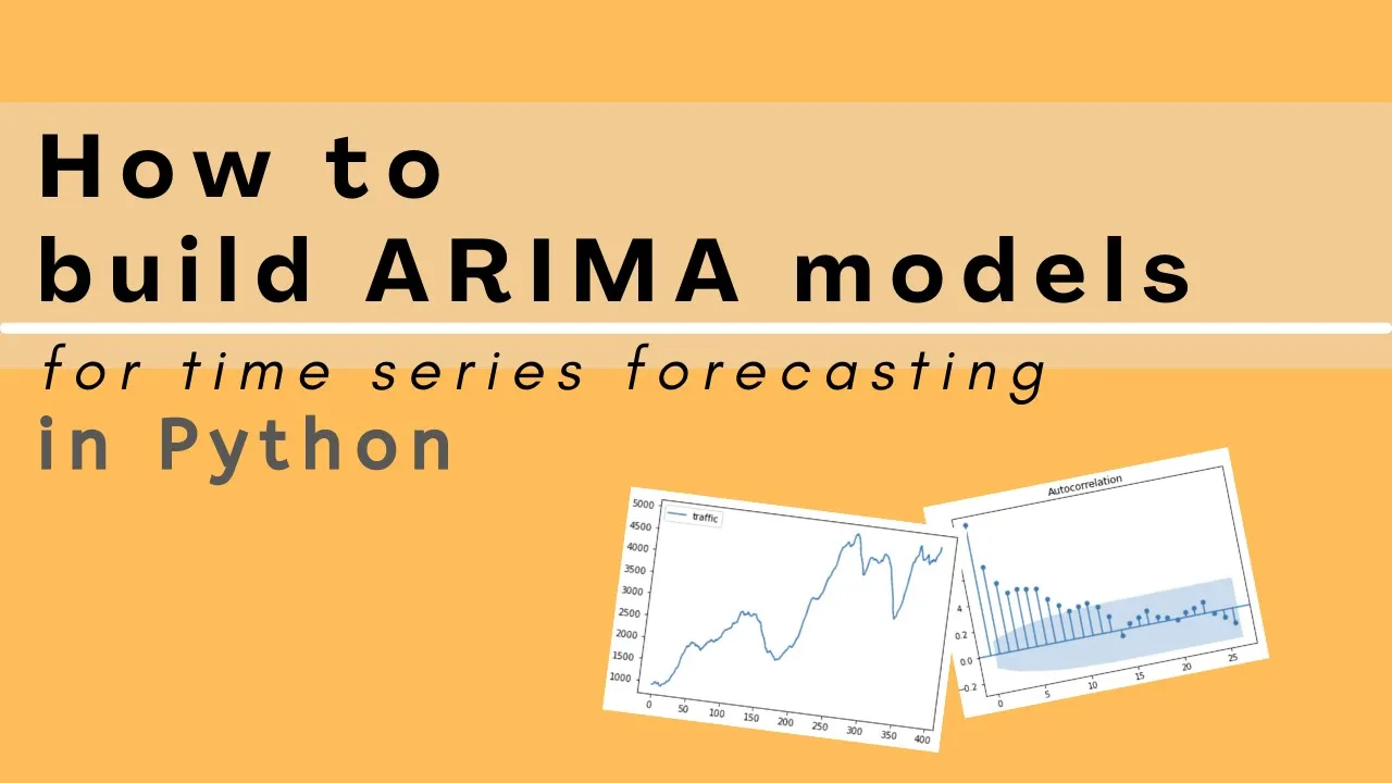
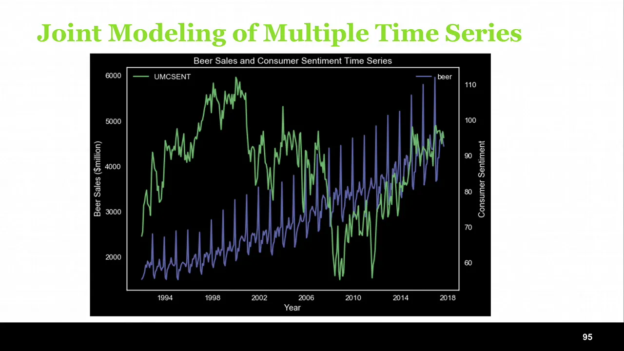
This lecture covers advanced time series forecasting methods including Vector Auto Regression (VAR), Vector Auto Regression with Moving Average (VARMA), and Vector Auto Regression with Moving Average and Exogenous factors (VARMAX), along with Seasonal ARIMA (SARIMA) and Seasonal ARIMA with Exogenous factors (SARIMAX), demonstrating how these multivariate approaches improve prediction accuracy by accounting for interdependencies between time series and external factors like holidays, compared to univariate models that only consider single variables.
Advanced Time Series Forecasting with Prophet and ARIMA Models
Added:Understanding of core time series components, specifically trends, seasonality, noise, and the concept of stationarity.
Familiarity with exploratory statistical tools for sequential data, such as Autocorrelation Functions (ACF) and Partial Autocorrelation Functions (PACF).
Proficiency in Python programming, particularly using data manipulation libraries like Pandas for handling datetime objects and resampling.
Basic knowledge of classical regression analysis and how model residuals are evaluated.
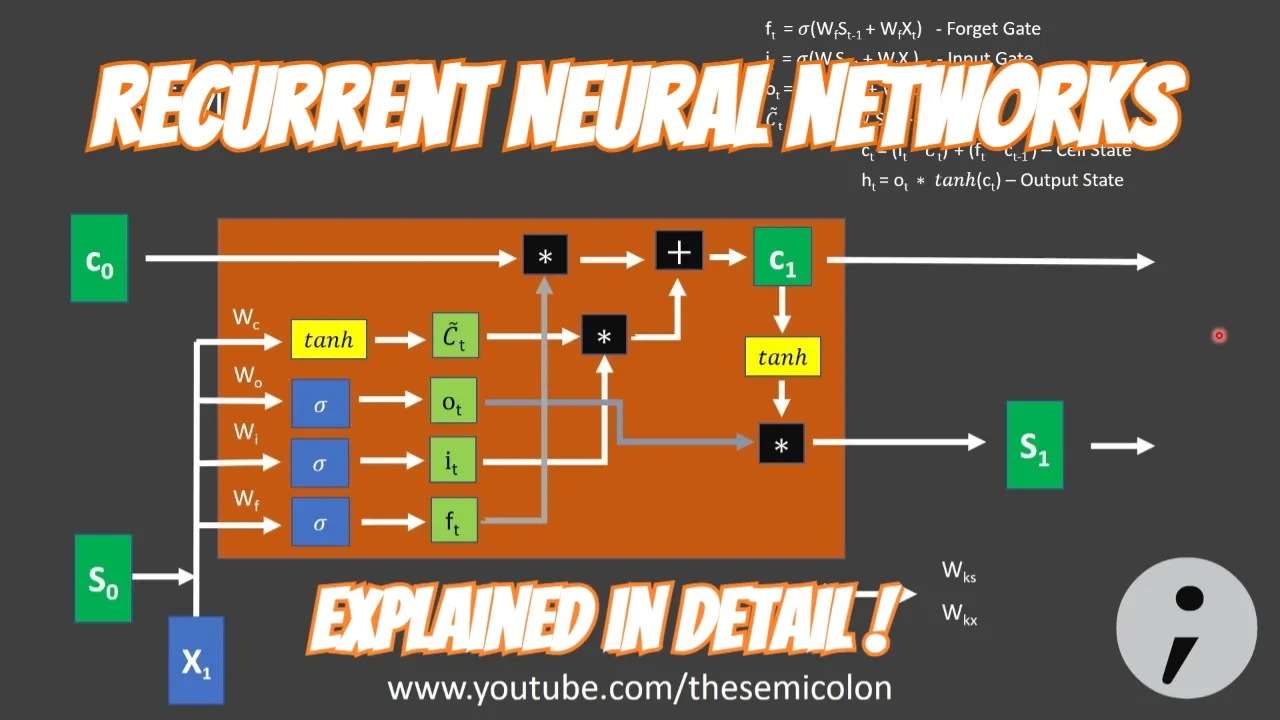
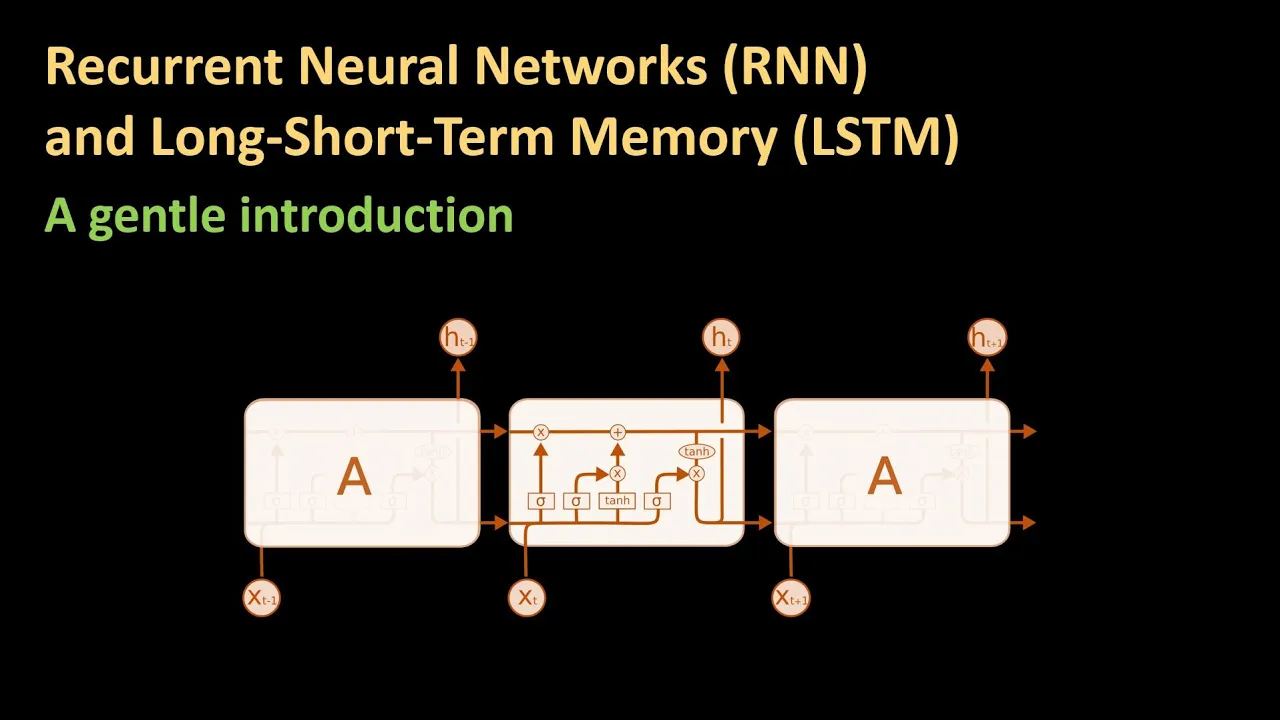
Deep learning architectures specialized for sequential data, such as Recurrent Neural Networks (RNNs) and Long Short-Term Memory (LSTM) networks.
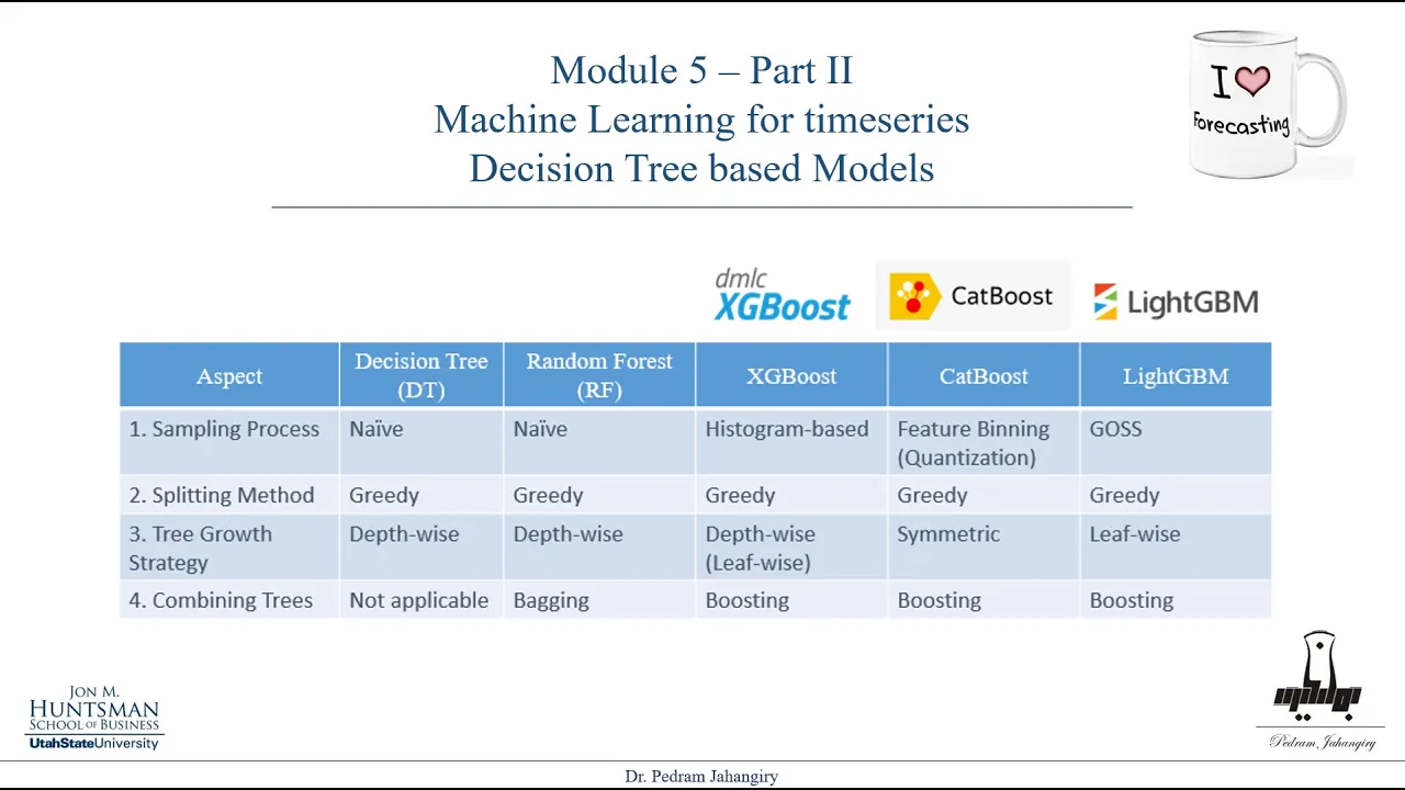
Utilizing tree-based machine learning algorithms (e.g., XGBoost, LightGBM) for forecasting via lag-feature engineering.
Multivariate time series forecasting methods, such as Vector Autoregression (VAR) to model multiple mutually-dependent time-varying variables.
Advanced evaluation and deployment strategies, including walk-forward validation (backtesting) and building automated pipeline workflows for production.
1.3K views37likes3:11:13Original Release: 2022-09-24
okay let's begin so good afternoon everyone and welcome to Advanced forecasting methods by 360. EMG so broadcasting is quite used nowadays and we have been spending a lot of time looking at forecasting related data so we are moving towards more advanced forecasting techniques why are we moving towards these more advanced forecasting techniques because you have more complex data available nowadays now if you remember when we were talking about forecasting in your class we were usually looking at univariate analysis or something close to those lines okay univariate is where you have a single dependent variable and a single time variable right so univariate analysis is easier to do but now we are also seeing the rise of multivariate analysis within the scope of Time series analysis okay so today we'll be covering both univariate and multivariate Analysis all right aside from that aside from just having more complex data right you also have greater requirements you have greater requirements for prediction all right people are asking for more and more how do you say it they are asking for more and more accurate predictions right we have seen that especially when it comes to recent year the last couple of years we had covered 19. a lot of the covid-19 predictions were time series related we were taking a historical look at the patterns of other diseases right we have taken a look at diseases like Spanish flu right we had other forms of bird flu that have come into the picture we also looked at SARS so we were taking a look at the historical timelines of these uh diseases and we are trying to use it in regards to covet 19.
okay so we are facing a greater need to be better at forecasting now forecasting is a very difficult task anybody who has spent some time on forecasting they would have realized that it is a very difficult task okay all right so in regards to this complication right we are trying to enhance our forecasting skills and this enhancement will help you a lot right when you are naming these Talk of the line algorithms especially we'll cover three very unique algorithms okay they will be a little difficult to understand at first but they are very unique algorithms so this will help you a lot you will also die spend a lot of time in Auto regression Auto regressive models now obviously I hope everybody is familiar with auto regressive models right what are Auto regressive models in time series concept right so we'll be focusing on these things okay so let's look at the agenda for today so these are the various models that will be covered today we have Vector Auto regression that will be the first concept we'll take a look at Vector Auto regression then we'll be taking a look at Vector Auto regression with moving average okay moving average is another concept that we had covered in a data science course how do we calculate moving average for uh let's say if you have odd number of uh observations how do we calculate moving average how do we calculate for even number of observations if we have taken even number of observations right so we'll be looking at Vector Auto regression then we'll be taking a look at Vector Auto regression with the moving average concept then finally we also know that time series data can be affected by exogenous factors what is exogenous factors here exogenous factors are factors outside of control of anyone okay outside are control now if we simple simply have a Time series data we have some time variable here and we have some dependent variable here we cannot say that there is nothing in the world that is affecting this dependent variable right there will always be some sort of impact let's take an example of stock prices right stock prices now when it comes to stock prices there are a lot of factors that are affecting this stock price right we are just not looking at time and the price we are trying to spend some time on understanding what else is happening why is stock price changing so much right so that is also very important okay so let's uh let me give you a very good example here just for a second let me give you a very good example for stock price now uh there was a organization called blizzard okay blizzard was blizzard it is still an organization but it also was an organization so blizzard is a gaming organization they produce video games okay so here you can see the kinds of Game World of Warcraft Diablo 3 Starcraft all these games have been produced by them okay they have also involved in uh Activision Blizzard so if anybody has played Call of Duty or heard of Call of Duty you would know the blizzard name Activision Blizzard so I'll show you uh this stock price so if we look at a one-year data right we observe that during this one year period there was a specific time here if we look at this time this time here their stock prices basically Tanked okay they fell by almost 20 dollars that is a huge huge fall okay more than twenty dollars you could say okay here you if you notice it is probably below 60.
the 52 week was lowest was 56.
so they they were averaging around 80 at this time frame and then it fell off to 56.
now if we are doing time series analysis for stock price prediction right what you would have you would have the time variable then you would have the stock price okay you take the time from uh one year ago today that would be what 17th August 21 up until 16th August 22.
you would look at the stock price starting off with let's say 83 dollars and ending nearly 81 dollars in between you have 365 days of Records right now if you are doing time series analysis you are trying to predict for the future price the time series model will take this fall into the picture right it will take this time fall in the picture like why did this specific event happen it happened it is not going to question the why the why is irrelevant to it right it will only make the predictions based on this historical data so the prediction might look like something like this then some fall and then Rising again correct that's how the prediction would look if we are making a very accurate prediction based on the historical data it will say that after two three months there is going to be a decline but what happened here was the CEO of this company was caught making let's say very bad remarks what sort of remarks you can explore that on your own at your own risk because whatever he said was not something we should discuss in class openly okay so he was caught making those remarks so there was a huge controversy involved surrounding him at that time frame at the time frame when the stock price happened right so what does that uh what does that remarks what is the controversy related to this that is what his this is an external Factor correct this is an external Factor so we are also going to try to account for these external factors okay we are going to try to account for these external factors because these external factors are clearly affecting our time series model okay so accounting for external factors becomes very important there are many many many examples where time series models will fall short of the actual prediction simply because people did not account for external factors so these external factors are as they are known within the space of Time series models as exogenous factors are extremely important towards understanding and towards the future prediction of external factors sorry towards the future prediction using the time series data okay so we have to account for these things okay once we are able to account for these things our predictions will become more accurate Okay so this is what we'll be doing okay so this is in regards to the first three Vector Auto regression Vector Auto regression with moving average and bar Max Vector Auto regression with moving average and exogenous Factor okay so always remember that if somebody is saying exogenous factors what do they mean they mean external factors external factors that are affecting your time series model but you are not accounting for these external factors we are not accounting for these external factors when we are normally building a time series model but now it is becoming more and more important okay and anytime this is a universal rule for data science anytime you come across a situation where people are starting to build more and more complex algorithms that you feel like are not you know required just take a step back think about something complex data complex data what is the meaning of complex data foreign there are a lot of complications involved with that data and just looking at the data and understanding the data is never going to give you the full picture you also have to look around the data what is happening in the data and this is where your research comes into the picture when you're looking at any data now let's say for example if we go back to our example of Blizzard Entertainment foreign variable and I give you the stock price you how many of you honestly like there is nothing wrong with giving an honest answer how many people here honestly would have research on Blizzard Entertainment before building a time series model how many people would have looked just outside of the like outside the data that is provided to you uh honestly like I'd like some responses now let's see how how active our session is we have uh 41 members so quickly you guys can reply in the chat window if you don't want to reply uh publicly you can just reply to me privately but I'd like to see some responses how many people would have actually researched on the data that is given to you 30 percent not always we are not always researching into the data sometimes you know laziness takes over you just look at the data you understand the data and you move forward and that is that is the harsh reality this is nothing like it's you know it's not like a personal slight against anyone I also do the same thing sometimes I look at the data and I start working with it I don't understand the data okay so I know we are only supposed to be talking about time series analysis but you know it is important that everybody everybody who is uh in this session or if you're talking to anyone always ask them to research the data as well ah we just see brief outlooks in the price chart we are just looking at the basic data right now if you guys weren't aware of what was going on in the background what was the actual reason for anything that happened right we'd be a little clueless right now if you research the data and then you research around the data right a quick five minute research on blizzard stock price around that time frame would have given you a clear idea of what is going on correct it would have given you a very clear picture what is going on and if you are taking part in some sort of competition or you have a competitive job interview or anything like that it's things like this that will make you stand out okay you are competing with people who are very good at model building okay so are you you are also good at model building but what is your unique point why should the organization choose your model over the other model why should the organization hire you over that other person it's these small details this attention to detail that is going to make you stand out it's just not knowing the fanciest algorithms you also need to understand the fanciest algorithms and you also need to put in extra effort everybody will appreciate that extra effort right when you explain your model why you build a certain model and then you explain it properly and then you give reasonings then you tell them that you researched outside of the data around about the data you try to understand it properly right they will be very impressed because you are paying attention to the details and the details become very important okay so this is lesson one of today's session okay pay attention to the details anytime somebody gives you any ml related work you're in a job interview you are working for an organization okay you are CEO of an organization pay attention to the details okay this is a very important factor all right moving forward what was the full form of arima anybody anybody harima anyone what was the full form of arima right arima was what Auto regressive with integrated moving average okay so here you are already accounting for moving average in Vector Auto regressive we were not accounting for this moving average so we moved into Vector Auto regressive with moving average same thing we are doing here in arima in arima we were already accounting for the moving average all right after this people worked on the Ariba models and they worked on advancing them further so they came up with sarima what is sarima sarima is seasonal autoregressive integrated with moving average so here we are also adding the seasonal seasonality as a very important factor we are taking seasonality as a core principle of this model okay now you have added seasonality to your arima model has your model improved would you say that your model is going to be more accurate yes it is going to be more accurate it's good to see so many people answering about Auto or email good work okay but is auto regressive now your model performance should have improved because you have accounted for a very important thing in seasonality what is the other thing that we can account for maybe something like external factors correct we can maybe account for something like external factors we can include these external factors okay so then we have seasonal Auto regressor integrated with moving average and exogenous factors exogenous factors are nothing but your external factors okay then we have TFT TFT is temporal Fusion Transformer TFT is a very advanced algorithm it is a very very Advanced algorithm and this is based on neural networks okay this is based on neural networks so this is something we'll cover we have FB profit that is Facebook's profit this is another time series model and this is by Facebook open source and then we have n beats n Beats to a large extent is probably considered the most advanced time series model okay we were not supposed to be discussing this but uh I have added it in the session so it might be a little complex because this is pure neural networks this is based on pure neural networks we are not doing anything else we are not using any other Concept in this this is purely based on neural networks okay so this is quite Advanced there is a competition called M4 forecast competition so uh in this competition I think it is yearly or something like that so whoever won the M4 uh forecast competition had a very high accuracy and N beats was able to beat that accuracy by three to four percent now three to four percent some people we might think that just three to four percent what's so special it's the difference between you know getting 90 percent and 95 in your exams just five percent what's the big deal right or for you know uh people if you want to understand in a different way 33 and 32 percent it's just one percent what's the difference what's the difference right it's just one percent right so career destroyed career would have probably be destroyed at 33 anyways but just saying that even a single percentage of improvement is quite a big deal right when you're working as a data scientist you will be spending days weeks months trying to improve your model from 85 percent to 85.5 percent so excess log to improve your model accuracy okay you have to get very creative very Innovative and that's what these models are creative and innovative okay so now that we understand the importance of Time series models now that we understand what all we are going to cover let's move forward so we are looking at Vector Auto regressive models what is Vector Auto regressive model it's a multivariate forecasting algorithm multivariate forecasting algorithm we are looking at multiple time series models okay we are trying to see how these two or more time series influence each other let's take an example of two or more time series that might influence each other we have a data foreign series so you're accounting for multiple variables Okay so let's say we have time frame here and we have covet how influential covert was we have time here then we have jobs how many total jobs are in the market how many jobs are available in the market would be can we say that kovit had a direct impact on this definitely right so it is a forecasting algorithm that is used when two or more time series influence each other that means multiple time series algorithm multiple time series are present and they are influencing each other okay so then what are the requirements you need a minimum of two time series there has to be at least two how can we check if two or more time series are influencing each other if we have just one time series correct and the correlation has to be there there has to be a correlation between these two Time series correlation must exist so you might be better off checking if correlation is present or not okay so how do we build a vector Auto regressive model we use step by step we go first you understand the characteristics of the time series that we are looking at okay whatever time series we are looking at will try to understand its characteristics okay then we test for correlation okay we are going to check if there is correlation between the time series or not then we check if the data is stationary or not stationary test so so far what we have done if we were talking about let's say for example we are talking about crisp MLP methodology what steps have we done so far data pre-processing and EDM we have taken a look at data pre-processing as well as EDM okay after we check for stationary if the data is not stationary step 4 would involve making it stationary okay so we are still not yet at a algorithm we are still not yet made our algorithm okay so we are still working with the data we are still trying to understand it okay then we try to find the trend Next Step would be trying to understand and find the trend okay then we go to our model building stage so if you follow these six steps you can use Vector Auto regression okay why are we using Vector Auto regression because we are creating lag okay we are looking at lag and we are saying that the future predictions will be related to the previous predictions lag concept is clear to everyone I'm not going to explain it but I'm just asking is lack something that is clear for everyone you if you don't know lag please focus on it okay so we are simply saying that each variable is a function of the previous values okay there has to be some sort of understanding that we are doing of the work we are doing there has to be some level of understanding right so it is important for us to say that each variable is labeled as a function of its past values okay so you can also use the variance covariance method so this is another method to use Auto regression or we can use Monte Carlo method so this is something these two methods is something I would ask you guys to do research at least Research into this at least understand what are these methods okay all right then this is Vector Auto regression after Vector Auto regression we come to Vector Auto regression with moving average what are the conditions and there must be a minimum of two Time series correlation should be there the time series are not stationary and we are here talking about the lag effect and the moving average effect okay so let's say I am talking about moving average I hope everybody is aware of how we calculate moving average we are talking about odd or even right if you have five and four you would simply calculate let's say y took minus 2 y minus 1 y y plus 1 y plus 2 over 5. you are basically taking the average okay so in Vector Auto regression with moving average we have started taking into account are moving average as well so this is going to improve the accuracy of a model okay so then we have Vector Auto regressive moving average with exogenous factors this is where you start coming into external variables so the concept builds upon each other if you are able to understand Vector moving average sorry Vector Auto regressive and you know Vector moving average concept you come to this correct we come into this then we take into account exogenous factors okay once we account for exogenous factors we come into governments so this is the basic introduction into these three concepts all right so now what we'll do is will spend some time looking at the code so just give me a second foreign okay foreign just a minute all right so we'll be taking a look at Vector Auto regression Vector Auto regression moving average and Vector Auto regression moving average with exogenous factors Okay so first as always you start off by importing the basic libraries numpy Panda stats model stats model is the library on which we are built a vector Auto regressive okay and we'll be using date tools okay so let's execute the code just um this annotation tool is messing up foreign so this annotation tool has been a little annoying so let's import all our libraries will use warning and will filter out the ignore warnings because you know nobody wants to look at the ignore warnings so we are going to do multivariate analysis and we'll be looking at economic growth okay we'll be looking at economic growth all right so we'll be loading the data from stats model itself so stat model has uh data set and we'll be looking at it so let's run this so this is the data so you're looking at the year you're looking at what quarter of we are looking at then we are looking at a lot of different factors here we are looking at GDP gdps the gross domestic product then we are looking at cons pounds is your income okay then you are looking at inv investment then we are looking at the government expenditure okay this is how much the government is expending expenditure then we are looking at DPI CPI a lot of factors are there you're looking at unemployment rate population inflation real interest rate so all these concepts are there so this data set is available in stats model if anybody is interested they can they should probably explore this there okay then moving forward will create a copy of this data and then we'll take a look at data types all the data is in float even the time doesn't float would it be okay to have time data as float no so will convert it into date time okay okay so let's run this and once you see the output it will make sense so look at the date time you have the year so what we have taken here is let's say we have one year 1959 okay now here we are looking at quarterly data quarterly data is nothing but your three months of data okay so we are not looking at the economic Financial quarters we are looking at the yearly quarter so you have quarter one two and three and four this is what gen too much April May June July to September and what October 2 December so what we have done here is we have taken the data we have converted it into integer okay we have taken year and quarter we have converted them into int values we have removed the float concept then we have converted them to string then we have created this variable called quarterly so what we have taken is we have taken the year plus q q is the quarter plus the actual quarter that is there so this would look like 1959 q1 1959 Q 2 this is a single column this is not multiple columns you are looking at single columns and then using date tools we are converting it into a date time format so we are taking the last day of every quarter okay so okay so we are going to be taking yes so the date tools module is able to understand q1 Q2 Q3 Q4 as quarters so it is able to understand that we have a quarterly data it is inbuilt inbuilt this work is done and it is taking the last day of each bottle because obviously these economic parameters will be measured at the end of the quarter will not be measuring them at the start of the quarter even if you take at the start of the quarter it will be the last quarter's data right so in order to account for the current quarter we are going to be moving with the next quarter data currently we would be in quarter three okay so anyways the library date tools module is able to take the dates from string okay it is taking the date from strings and it is converting them into date time format okay so this is the basic preprocessing step that we are doing with the data sets then what we have done here is we have taken some factors we have taken some factors we have taken real GDP real cons and real investment okay and we have created it into a separate column but before we do that let's check for relation okay we'll check for correlation what is zero cells foreign we cannot do correlation here so what we'll do is we'll run this cell so here what we have done is we have taken df2 and df2 what we have done is we have created a new data frame that we will be using for our Time series okay we have looked at the factors we have again right we have this data now this is where your research comes into the picture you look at this data and you try to figure out the most important factors for economic growth okay so we'll be taking real GDP real income and real investment okay so we can check for its we can check for its correlation because these are all numerical columns so as you can see that we have a very high degree of correlation it is basically perfect correlation correct and then we'll add the time series time index to it and then we'll take a look at the data so now we have the data the date and we have the income we'll plot them so this is the plot if we had to Define the trend here the trend would be basically upward right but this thing is not so upward the real investment is not improved since 1959 to 2009 but these factors have improved definitely from here to here the GDP and the income have improved okay so then what we'll do is we'll take the log to reduce will do transformation here okay we are going to check for variance okay we are checking for variance so here we can observe that in comparison to other columns real investment is showing a high degree of variance everything else is moving in a perfect order everything else is increasing at a linear order so that means if we spend some time looking more in depth into investment we'll notice that movement okay then what we'll do is we'll build our model with Vector Auto regression okay so you have these various metrics coming into the picture you are taking a look at information criteria and all these things then we'll fit them in our model and then we'll take a look at the equation okay so here you see we have tried for three different equations okay we have got the coefficients okay so here this is the equation to calculate real GDP these are the equations to calculate income these are the equations to calculate investment and this is the correlation Matrix of the residuals so as you can see that real investment is highly correlated its medium correlation to GDP not so much to income okay so let's look at the resulting plot all right so these are the resulting plots from that model and now we'll try to predict the next 20 quarters so here you can see that the prediction line is sort of straight look at the data look at the seasonality in the data and look at this right so basically what it is saying is that it can fall Within These lines it can fall within these lines okay so then we will add time series We'll add moving average okay so here specifying the order you're specifying p and B the seasonality and the the trend and the what was the the trend and the order seasonal difference order okay so if you remove the first value to zero this becomes a vector moving average model if you make the second value as 0 it becomes a vector Auto regressive model you need a combination of two for it to be considered as a moving average here now you might notice that we have taken VAR Max VAR Max is the library that we use to calculate both Varma and warm X but unless you specify the auto regressor uh the exogenous Factor it is not taken into account okay so then we'll run this and then we are going to run it for a few iterations we are trying to find the best possible model so we'll run it for 100 iterations so we'll wait for it to run it has run and then we'll take a look at the result okay so you can look at the AIC Bic you can look at the various equations that you are getting check for P value okay all these things are there you're looking at the square root then we'll plot the result so as you can see we are looking at investment is not converging for a longest time but these values converge quite quickly so that means investment is a issue here okay we can also try with diagonal error okay so let's look at this so again here AIC is reduced from the previous one right here you can see the convergence has still not happened but again these two are converging quite quickly all right now what we'll do is we'll take real GDP as the exogenous Factor we'll run this will let it run for some time and then we'll take a look at the model here you will notice that the AIC score has further improved okay so exogenous Factor has allowed us to improve our model performance okay so this is in regards to Vector Auto regressive models okay then moving forward we have seasonal arima okay so so seasonal arima is the seasonal iteration of the arima model okay so this supports univariate time series analysis thank you and measure the python for the codes I'll let you know before the end of the session I'll let you know Okay so it supports univariate time series okay where the seasonal component is included okay so if you have a seasonal component with your time series you are going to take this okay so you will also be taking into the account Auto regression obviously Auto regressive because we are using arima you'll also be taking into account the seasonality of the data that you are looking at okay so here we are going to look at something we call as the p d Cube now how many people are familiar with these terms PDQ okay so what is p p as your trend Auto regression so we are doing Auto regression here we're looking at the trend Auto regression B is your Trend difference okay so this is this is small P small D small cube what is happening it is working now maybe because you're not able to have it is working for you maybe some problem any issues with the voice are you guys able to hear me the ones joining only okay all right so you have small p small D small p is the trend Auto regression D is the trend difference and then you have q small q that is the trend moving average okay then you are also looking at Trend moving average thank you so this is PDQ then you also have something we call as p d q M so these are capital P capital D capital Q and capital M p is your seasonal autoregressor so you are not looking at Trend now you are also accounting for seasonality right so using PDQ we Define the trend okay then we have d which is the seasonal order difference okay then you have q again which is what seasonal moving average so PDQ basically the same thing the only difference is how you write it if it is small PDQ you are talking about the trend if it is capital we are talking about the seasonality okay and then we have m m is the time steps for a single season so let's say for example we are looking at data starting from Sunday to next Sunday and that is our seasonality how many time steps would be there for weekly data seven if you are looking at quarterly data like the data we are looking at last time how many how many time steps should be there in quarterly data four if you are looking at monthly data how many time stats time steps would be there 12.
okay so this is what we are talking about when we say time steps like I said for python code I will let you know in a little bit okay so this is seasonal autoregressive so again you're just taking the arima model and you're accounting for seasonality with it okay and then if you add an exogenous practice you come up with what you come up with what you come up with sediments okay so this is in regards to the seasonal Auto uh seasonal arima and seasonal arima with exogenous factors so again we don't have a lot of theory here to go through so we'll jump right into our codes okay so for codes just give me a second so here we'll be taking a look at sarimano so what is our use case here we are trying to predict daily customers for different restaurants okay we have four different restaurants and we are trying to predict the daily customers the daily football how many people would be coming to that restaurant on an average okay so here will import our data we'll run this code okay so what I'll do here is I'll show you the reason why we are taking index as date and why we are passing the date so what we can do here is we can also create another data frame so let's run this so all right so this is your data with date as your index column now if you're taking it without the data as your index column this is what it looks like you have date and you have this so just notice the difference in the format so we are parsing it in order to avoid a situation like this where we have to do additional pre-processing we are simply parsing the data and we are going with this okay then we are checking the frequency we are checking for null values we see we have null values at the end 39 null values so we'll simply just drop these null values and we are left with 478 entries okay because the N A values got removed okay here you can see ndn values now these n a values in Holiday name are different from these NBN values means that there is no holiday on that it is some kind of record n a n means that we don't have any information okay so that is the difference between the two then we'll check for other stuff we'll look at the data types we'll take a look at holidays are in 64. holidays in 64 holidays whether it was a holiday or not zero and one okay then we are checking for columns then we are going to convert this values into int values the total values into int values now if we look at it we have integer values let's try to draw the data can we make any conclusions based on this what would be the trend here upward downward what linear trend is there if barely any movement is there if we look at it but can we see the seasonality here properly like this seasonality here present or not obviously we cannot just Deep dive into it because we have a lot of Records but can we look at the seasonality here yes it is linear correct Edition yes so we are able to however see seasonality is present and because the difference in the peaks in the trolls is pretty much constant it is not multiplicative seasonality all right so let's look at the days when we have holidays okay so these are the dates now this is a america-based uh America based data set we are not talking about Indian holidays so obviously some dates might not make sense to us right because we are not familiar with that apparently they have a holiday on a lot of days that we don't expect all right so now we will account for the holidays now here we have the black lines representing holidays now you might notice that most of the Peaks are happening very close to the holidays correct most of the peaks of the data are happening very close to the holiday or on the holiday okay obviously some sometimes it will be different but most of it is happening around the same time here we have a thing here you don't have anything here we have the highest peak here we have the peak this is basically right next to that date here we have a very high peak so can we say that holidays are affecting the sale now here for example let's look at between July and whatever October between July and October here you notice that it is not very high but then the holiday comes around it is high near the holiday also it is high right can we say that holidays might be affecting our date time series data is that a conclusion we can draw yes that is a conclusion we can draw that holidays are affecting our time series data okay if we had not even looked at it right let's say for example we just looked at this data we said yeah seasonality is there some sort of trend is said would that be sufficient information foreign that would not be sufficient information we have to exam I'm sorry I'm not understanding what do you mean we don't know exactly when what are we talking about like we don't know exactly when the holidays are or when the Peaks are is that uh are you going along those lines foreign you have on your data the better it is okay now we will do decomposition thank you all right uh let me try to increase the figure size hmm okay let's just go with this I guess it's not applicable here so here we notice the total we are noticing the trend we can see the seasonality and the residual okay if we were taking a smaller data like let's say for example 10 or 20 we could probably also understand the seasonality in a better way okay but we know we know that the seasonality is present okay so then this is our seasonal plot the seasonality we can see here right so let's take a look at the data we'll split our data we'll take the last six weeks in the test data so we'll be taking whatever the last six weeks are so we can account for more data as well as some holidays so what test data is going on up until trained data is going on up until uh 2017 11th of March and our test data is starting from 12th of March and going up until the end of the end of our data set so here because we have a daily record we are going with weekly Trend weakness weekly time steps right we are going with weekly time steps so how many steps we are talking here we are talking seven steps so here we are trying to use a one zero zero four double zero seven model so you are looking at again PDQ and p d q m so you're looking at one zero zero and 4 0 0 7 model okay so you understand where these terms are coming into okay you can try it with different models you can drive it different uh what do you call it values you can also try maybe some sort of Auto arima model to figure out the best parameters and then you can take it okay but this m value has to be 100 correct the same value you have to take correctly we are looking at the weekly data so we have gone with this so let's fit our data so our P values are not very high our AIC score is this much so remember this AIC score okay right so these are the different kinds of lags we are taking with One lag with 7 lakh 14 lakh 21 lakh 28 lakh okay I hope this is understood that we are taking lag here all right then let's take the prediction values and let's plot these prediction values so here what are we observing our predictions are able to capture seasonality to a great extent right if we look at it yeah the orangish line is our prediction and the blue line is the total now here if you look at it we'll see that we are able to capture at least the seasonality to a good extent we are able to have the seasonality present have the seasonality peak where it is speaking so here it is speaking obviously there is a it's quite a difference between the peak data in our data almost 50 people okay but here if you look at it the act the prediction is pretty accurate for the second one but the important Point here is that wherever this model is at its lowest our predicted values are also at its lowest okay wherever the model is it's is it at its peak our predicted values are also at the peak so we have chosen a pretty good value for sarima we have gone with a pretty good value so obviously scope for improvement is there right this is not a hundred percent accurate model but it is quite accurate let's take into account the seasonality the holidays so here you can see that around the holidays the values are different they have to pick differently so we'll try to predict for that will try to evaluate the difference for the total for the test the mean was 134 the average footfall was what 134 for us it was 132 so we are quite close to it okay so if you look at the rmsc the rmsc is 39.
okay so we can say that on an average our prediction will be off by 39.
okay so it is not a bad way but definitely we can try to improve this all right so let's check the rmsc 39 now will account for exogenous Factor okay now we'll account for exogenous factors so here if we go scroll back up we have the Serima model and then we have the other metrics that we used to measure the model performance now let's run this again let's call it result one so we have some sort of separation so here now if you look at it we have taken into account an exogenous Factor now the exogenous Factor here is quite clear it is our holidays holidays are an external Factor affecting the footfalls of a restaurant okay we will keep the same sarima model because this model gave us a pretty good accuracy right so we'll keep the same sarima model but what we'll do is we'll take holiday as a external Factor okay so then we'll check for it so you can see that our AIC value has decreased okay again we are taking the same logs sorry same lags and we are also accounting for holiday in this scenario okay so the same thing we'll do we'll uh try to take the prediction and this is our prediction so the difference is within these holidays our model is now peaking higher but most of it is still pretty much the same because our model was already quite accurate okay we'll check with the this here now the difference is here we were this average footfall is not going to change the average would follow the actual data is not going to change okay but here you will notice I think I know I made a mistake here just give me a second let me clarify that so here we had to take results one okay we had to take results one because we had I changed the name here two results so that's why we are getting the exact same model so now let me just make sure that I am not doing any mistake here foreign curve has changed slightly the change is very slight the Improvement is very very slight but the change is there if you look at the previous model and you look at this model you'll observe that change okay now it is making a closer prediction to the peak based on the holiday here also here the peak is still there all right but will if we compare these two if we look at this one and then we scroll all the way up look at this one there is a slight change in the dynamic offer model okay so we'll see if we accounting into accounting for the exogenous Factor has made a difference or not it has made a slight difference the difference is now we are going over the actual average of footfalls so now maybe we are predicting more than the actual average because our model is taking into account holidays now so it is predicting more for holidays so then we'll measure rmsc and MSC so here our rmsc has improved our rmsc for sarima was 39 point something and rmsc for Siri Max's 31.
so our average prediction has improved in overall we have built a better model so once again taking into account the exogenous factors our models are improving okay then we'll compare the two models so here we can see the comparison okay then we'll build a model for the entire data we'll combine and we'll build a model for entire data and this is our forecasted value this is our forecasted value this part is our forecasted value we can compare it to this part Okay so you'll notice here that our Peaks are happening around holidays for our forecasted value so our model is able to understand the exogenous Factor obviously not all holidays are leading to Peak some holidays are leading to Peaks so it is able to make that prediction okay so it is able to understand that Trend it is able to understand that holidays are a important part okay so this is our forecast this is our normal forecast without any exogenous factors okay so if we look at the trend here it is quite similar to the overall trend we are seeing sorry the seasonality here is quite similar to the overall seasonality we are seeing so our model is pretty good but obviously there will always be some scope of improvement so this is sarima and Ceramics so any questions regarding to this any questions regarding to what we have covered so far anything that you guys are not able to understand electrical lag lag is when we are comparing the historical data lag is when we are looking at the previous data in relation to the current data we have taken lag right we've taken lag one lap to lag three like that we took it in when we are taking the class so let's say this is a historical data some values are there right we are trying to understand how the previous value is affecting the next value so if we are taking lag one this is what lag one would look like if we are taking lag 2 it would look like this sorry 100 and 120 so we are trying to see how the previous values are affecting the future values because we are saying that the previous values are what is going to predict the future values okay that is the concept of Auto regression and then into that we are also now accounting for seasonality so that is how we end up with seasonality okay so if we don't have any questions let's take a break we'll take a 10 minutes break and then we'll come back and we'll take a look at the other three concepts foreign okay let's uh continue so the next model that will be taking a look at is FP profit okay will not look at TFT first we'll first look at FP profit Okay so FB profit is from Facebook and this is used for univariate time series analysis the big advantage of FB profit is that it allows for automatic hyper parameter tuning okay so what are the advantages why are we using FP profit what is the reason aside from being associated with Facebook it also has other benefits okay just it's not just because it is Facebook related data first of all it also accounts for holidays so automatically without us having to specify it will account for holidays okay that is one advantage it is very useful with data that have strong seasonality and multiple seasons that means you are looking at a long a lot of data okay if you have strong seasonality and you're looking at multiple Seasons this is very useful okay and it is very robust towards missing data so if you have missing data in your uh data set it is very good towards using that okay so these are some advantages that we are looking at why FB profit is getting the hype that it is getting okay it is also very good at handling outliers okay so basically all the flaws that you might have in a data like outliers missing data it is quite good that accounting for those when it is making future predictions all right so this is some advantages okay by default so now how does it work okay it can take data in a very specific format okay it can take data in a very very specific format it cannot take data in any format you give okay the time Factor has to be renamed as DS okay the output has to be renamed as y so unless you give the names d s and Y FB profit will not work this can be considered as a limitation as well but this is how it is going to work okay by default it will use a linear model so it uses a linear model to make the prediction okay so these are some basics of FB profit it will also have a saturation point saturation point is also accounted for when we are doing FB profit in this saturation point is when you are looking at economic factors if you're trying to predict economic growth you will not have if you're trying to predict economic growth there is a limit to the economic growth right there is a limit to what we can achieve when we are trying to grow our economy so there comes a point let's say we are talking about investment by government you're taking into account population you're taking into account the interest rate on borrowings you can keep increasing the investment you can keep increasing the population you can keep your interest rate at a low point but that doesn't mean that your growth will be infining there will come a point where more investment will not yield more economic growth more population will not result in more economic growth right because why if your population is growing a lot then you also need to have jobs growing at the same rate if that jobs cannot keep up with the economic growth then there is no point of having more population right all you'll get up is a higher unemployment rate so the point where factors cannot increase the investment by a great extent is your saturation point so whenever you are looking at economic data you are always going to get some sort of saturation point so FP profit if you are working with the economic data it will account for that saturation point where is that saturation point it will predict that that is part of the prediction okay so that can be very useful when you are trying to explain some economic data set to somebody when you're trying to show the level of investment let's say an organization needs to make okay if you are using holidays if your data set has holidays right the columns have to be named as holidays they cannot be anything else they cannot be named as leaves let's say for example they cannot be named as leaves or vacations or they cannot even be named holiday they have to be only named holidays so time has to be as BS output has to be as y okay so this is what we try to do in FB profit the names are very standardized they can be useful they can be helpful because we are looking at univariate data you are looking at one time variable in one output column so it is easy just to rename the columns as DS and small y holidays have to be named as holiday if you are trying to account for holidays using FB profit you need the exact dates okay you need the exact dates in your what in your historical data obviously this data will be available if we look at the data set that we were using for sarima and sarimax we had already had this historical data accounted for okay but you also need the exact dates for any future prediction for any future prediction you need to have these exact dates okay you can also factor in for multiple holidays let's say for example we have three or four holidays for Diwali right you can also account for that if you have a whole set of holidays in foreign countries you might have Christmas break where people are on a week-long leave right that is also something that we can account for okay and another advantage of FB profit when we are using it in regards to Holiday okay it has country specific holidays whatever the holidays are for that country it has those holidays available okay so this is in regards to FB profit now we don't have a lot of explanation to do here simply because we cannot keep explaining the same basic concepts of Time series for every of the every one of these models right so these models are quite simple to understand so now let's take a look at uh FB profit profit so for FB profit we are using car sales so we'll take a look at the data set now this is an important thing to remember you need to use pip install profit for this to work okay sometimes you run into issues regarding the installation so in that context you will use Fonda installation so whatever the content installation is you can use that Okay so don't use every profit or don't use anything else you simply use profit okay pep install profit previously I think one month back it was pip install FB profit but now they have changed it to profit okay then we'll import our data set we'll look at the data set so our data set is something that is already okay DS um sorry the chat window doesn't pop up on this system BS is nothing but your time data okay DS means nothing but your time data so whenever you're looking at time data this is what it is given as the model is automatically going to do the model is automatically going to it is not handling the missing data it is robust towards missing data what it means is that the one second keep an eye on the chat anytime anybody asks a question just let me know because I'm not able to see the pop-up here this is Linux so the configurations are different you can't even use epic randomness okay so DS is nothing but time series so how it is not handling the missing data it is not doing anything to the missing data what it is doing is it is making sure that the missing data is not affecting the future prediction okay if you have any other algorithm if you use that then you will get into the trouble but here that is not a problem an economic factors are basically anything that is affecting your economy okay we can talk about the GDP we can talk about the investment private and public investment we can talk about the average salary of a person okay we can talk about unemployment rate employment rate okay all these any any metric that is going to affect your economy the national economy the Country economy is known as economic Factor all right so moving forward we'll take a look at the first five and the last five rows and then we'll plot the data so seasonality in Trend what is the trend here foreign Ty do we have Trend here friend is here upwards the trend is moving upwards seasonality is also present okay seasonality what sort of seasonality are we looking at multiplicative or negative here it would be additive because the difference between the Peaks and the trouser is not increasing here we have a specific time frame within which it is increasing but if we look at it afterwards as well it is pretty much the same okay so it is additive seasonality then we'll make it into a date time we'll convert our column into date time okay so date time changes the format okay it changes the format this was DDM month date month year but we need it to be here date month okay here you notice that the date is always the first the month is the one that is changing and the year is also changing so we are looking at data from 1968 so from 1960 to 1968.
okay foreign next we'll take a look at all the factors that are all the parameters that are present in profit so you have these attributes you also have ad country holidays add group components add seasonality construct holiday data frame logistic growth so plenty of different parameters are available and you can explore these parameters and you can try to use any of them okay these are all valid so let's build our model we'll make sure that the column names are same okay we'll fit our model the model has been fit in a data so additive yearly weekly these are the components these are the different components that are available to us okay so the next thing we are trying to do here is we are trying to build a data frame for the next year we are trying to predict the next year every profit allows you to do that okay so we have the next year available to us then we make the prediction and this is our prediction so what all can we see here we are looking at the trend y hat lower y hat upper what is this this trend is here prediction the actual prediction value what is y hat lower y hat upper this is the upper limit and the lower limit okay they are saying that the prediction should fall between these points okay this is the this is accounting for error you're looking at Trend upper and lower you are looking it in additive terms okay you're looking at in additive terms weekly lower upper then you are looking at multiplicative term and then finally we have a so this trend is not the prediction my mistake there we have our actual predicted value y hat this is nothing but this y hat we have already seen these uh values before okay so this is a predicted values so then we'll plot for these predicted values so here because we have it is taking a seasonal Trend that's why it is looking like this okay so here you can notice the weekly trend the yearly right so all these values we can take then we'll use cross validation we'll initialize our cross validation process and then we'll check for the performance Matrix so here we can see that are models in accuracy is around 70 percent we are accounting for 17 accurate in accuracy so you are getting around 83 accuracy so definitely there is scope for improvement okay there is definite scope for improvement so then this is the actual value versus the predicted value so you notice that it is not as accurate so this is one of the drawbacks with FB profit okay I've always found that the accuracy is not the best okay so whenever you're trying to use every profit this is something that you have to account for the last time I use this we were getting around 33 percent inmate so the error was 33 Okay so this is FB profit it is useful but it also has its drawback then we have two neural network based algorithms the first one is called as temporal Fusion Transformer so why are we the first question is why are we moving cross validation is done the same way you do cross validation in any other algorithm we will always have some sort of hyper parameters hyper parameters these are not the same parameters these are not the same thing as parameters you are using hyper parameters these affect how your model is built you can try out different hyper parameter techniques and based off of that you will get your improvements or not improvements okay so you will have to find hyper parameters for whichever model you are building and it will do the cross validation for that cross validation is nothing but hyper parameter tuning okay next we are looking at temporal Fusion Transformer now why are we moving towards neural network based we are moving towards deep neural networks we are moving towards AI Concepts why is this move happening okay because again data generation has improved the amount of data being generated has improved a lot okay so if you have let's say a electronic electric company previously in the older days they could not account for a lot of factors because it was not possible [Music] okay now you have something called iot sensors these sensors are sending live data back to the company they are capturing multiple things they can capture the environmental factors as well real-time environmental factors if there is an outage how that outage is coming they can also use these environmental factors to make further predictions right you are looking into an accounting for multiple things so many different factors are coming into the picture that the data being generated again is getting complexer okay so you are looking at a huge collection of data you are looking at multivariate data okay you're looking at multivariate data that is uh what do you call it that is also from different sources so the origin Source might be different for different data right and you have a lot of external variables being accounted for now if you are trying to use ml based algorithms in this it will be a problem because ml algorithms will not be able to cope with this so this is where we are moving towards neural networks neural networks are better at handling more complex data foreign taking a look at portfolios investment portfolios investment portfolios are diverse they include stocks they include bonds you know they can include real estate it can include things like gold okay so you also have mutual funds so you are looking at a lot of different factors that are affecting your portfolio so in order to predict your portfolio you have to account for a lot of things and while accounting for these things you also have to account for factors individually affecting these portfolios right you have to look at maybe the stock market on a daily basis right bonds issued by a government you have to look into the government practices real estate prices what is affecting the real estate price what is affecting the gold price all these things you have to account for so again you are looking at a really complex data that you have to use okay so this is where time series this is where even time series data is becoming more and more complex foreign Fusion Transformer is a attention-based deep neural network now I will not bore you guys with the details of uh thank you the attention-based deep neural network but the advantage is this is great for performance and interpretability so the performance is very good and it is very interpretable so you are able to understand a lot of the information better okay so see uh yes let's take a slight detour here now cross validation can be grid search can be random search there are also other methods like Biogen search as well as something we call hyper op so you are looking at various different ways of finding the best set of parameters okay so let's say our model has four hyper parameters we are trying to tune okay so parameter one has four values we are taking parameter two halves eight values we are taking parameter three has five values we are taking parameter four has ten values we are taking so what we do in Cross validation is we take each combination of these parameters and we try to build a model what happens is grid searches this is let's say for example a grid of a possible parameters all the possible parameters grid search will start with the first combination and it will keep going up until the last combination so if you have 100 competitions 100 combinations grid search will run for 100 times if you have 10 000 this will run for 10 000.
that is not the case in random search in random search it will randomly pick up some combinations and it will try to do those combinations okay it will randomly pick there is no specification that we are doing so out of 100 combinations let's say we put the limit to 50 it will take 50 combinations and it will give us the results these 50 combinations are taken at random so the advantage for grid searches it is more accurate and this is faster the disadvantage is that this is computationally very very heavy okay but this is again not that heavy because it is moving at a faster speed so this is the difference between uh wait what happened here meeting I'm in the meeting get the session end Voice is coming okay I don't know what's going on here um sorry for that so like I was saying that great search it will search for every single parameter there is random search will randomly select some parameters and it will go for it okay so this is the difference between grid search and random search so grid search is more accurate but it is slower random search is less accurate but it is faster we also have a lot of different uh techniques that you can use there seems to be some problem with my zoom meet okay what is he saying are you able to hear it yeah can you hear me sir hello all right no problem so you can continue with it just a second yes just a second okay foreign cross validation and stratified so similarly what methods do we have for time series I was asking you so yes as such we don't have any specific uh hyper parameter Tuning In Time series okay we just use what do you call it cross validation or sorry we are using in Cross validation we try to use these grid search or random search okay that is always the best option to go for okay what if I mean what if we have an imbalance data set in that case uh in imbalanced data case we try to use try to make it balanced okay I mean without and prior to that we need to do I mean yes using cross validation we can't do no no cross validation does not affect the data it only affects the model building stage yeah yeah like uh yeah okay okay cross validation does not affect our uh what do you call it the data it is only going to affect the model building stage okay okay so all right so we are looking at uh temporal Fusion Transformer right so it is very it the performance is quite High and it is very interpretable that means you can interpret what you are doing it so we'll look at the benefits the benefit is that it is rich in features that means it is going to support three types of features we are looking at temporal data temporal data is time-based data with in known inputs for the future so we know the inputs for the future as well okay we know the inputs that we are going to take in the future then it will also support data where the inputs are known only for the present data only for the data that that is present for us we know that and it will also take care of exogenous factors okay so it will take care of any exogenous factors okay then heterogeneous time series so you can train multiple time series here you can look at multiple Time series and each if you are looking at the data from different sources you can use multiple time series here okay so you have to remember that multiple time series is not the same thing as multivariate Time series okay this is a very important point that you have to remember that multiple time series are not the same thing as multivariate Time series okay then it supports step predictions so basically you can have predictions done in a step phase manner okay so you can have intervals you can create intervals and within that interval it will make the prediction okay again it is quite interpretable because it is a attention based deep neural network so all attention based deep neural networks are quite interpretable okay it is high performance it has outperformed models like arima okay it has also outperformed models deep neural network based models like djr dprs Amazons uh uh Auto regression model then you also have another model known as mq RNN this is a lstm based model and you have deep space State model so it has outperformed these models so it is again one of the best models that is available okay and the documentation is quite available the documentation is quite detailed and it is available quite easily so it makes it easier for us to perform the scenarios now we will understand you can use TFT with either tensorflow or you can use it with pi torch okay so you can use it in either so this helps people who have preferences uh tensorflow is easier to understand for people who are not familiar with tensorflow and Pi torch tensorflow is again easier to understand but it is slower Pi tots can be a little complex at time to understand especially when you are starting out but it is faster okay so that is the difference now we'll take a look at the code because it will be easier to understand when we are taking a look at the code so to use TFT we are going to use a library called Dutch darts is a very useful Library when it comes to time series analysis okay that's that includes a lot of different model it includes arima models it also includes a lot of deep neural network implementation okay so why are we using dot because it makes it easier to unders to like back tests or models okay if you want to perform back test on our models you can use it it also uh you can combine predictions so you can combine different predictions into a single prediction so when you are dealing with multiple time series data this is quite useful okay and it also takes into the factor external factors so external factors are also included okay so darts is quite useful so that says one library that a lot of people are using for prediction so here we are using time series we are using scalar we are using TFT model we are trying to check for seasonality Trend and seasonality May we are using the they also have a data set here passengers data set so they have a lot of useful information available in them okay all right so let's look at the code the code is fairly long so it will take us some time to go through it so first we'll import all the necessary libraries what just a second let me just give me a second you would touch Okay so maybe it is opened in the wrong environment just give me a second foreign okay so it was open in the wrong environment that's why this was not working so we are using dot shape all right then we'll load the data okay so we can take a look at the data set so the data set is in Array format we have a data set for 12 months okay it is in a date array format okay then we'll convert it into a data frame so this is our data starting from 1949 and we have the number of passengers the number of passengers is in thousands so that means whatever number you see you multiply it by a thousand okay so this is an Australian airport so we are taking a look at how their data is growing how the number of users are growing for the airport itself all right so then we'll plot the time series upward strength what would be the seasonality here what type of seasonality Are We noticing here anybody anyone what type of seasonality Are We noticing here it is multiplicative we are looking at multiplicative seasonality okay so then let's continue we are checking the seasonality and we are checking for the first we are checking seasonality from seasonality of 2 to 6. so is it seasonal true it is seasonal what is the seasonality it is an order of 12 months okay then we'll check for Trend components and seasonality components yep so this is the seasonality then we'll Define the date this is our date we are taking 1957 1201 as our training data so then we'll split the data we'll transform the data using scalar we'll create covariance we'll check for covariance between the year month and integer okay now here we are creating our txt model so this is where the uh becomes so here we are pushing 32 points into our model at a time and we are saying that you can give out 36 the hidden size this is the hidden neuron hidden neurons how many hidden neurals neural networks are available you have two lstm leader layers what is the dropout dropout is after each iteration how many data points do you want to drop out so we are saying 0.1 then we are keeping the batch sizes 32 at each batch will be of 32 then we are using quantile regression here we are setting the random State at 42 and we are saying Force reset is true so these are some various factors that can affect your TFT model so we'll run it and we'll set it so it is going to start training so the important thing to keep a point here is the training loss as well as the overall loss if it is reducing then you are using the model properly if it is not reducing then you should probably stop foreign so now that the model has run for 500 epochs what we'll do is we'll check if the predictions are accurate they also have a measure they also have a way of checking if your predictions are accurate or not so they are loading up the data and it is saying that yes the predictions that we have made are accurate we are not drawing any uh inferences we are just saying that these columns are related to each other because that will be that will be used in the future okay so we are just defining that the columns are related to each other we are just checking the covariance between the columns we are not drawing any conclusions from them then we are going to create function this function is going to plotter predicted value we are going to Define these quantils These quantiles are the range for the upper and the lower limit okay so we'll Define two functions here and then we'll perform a Time series so here this is a time series model that we have built so as you can see that are mean absolute percentage error is only three percent so our prediction values are only off by three percent so here we have the 99 percentile bank and the 90th percentile band so here it is difficult to see because it is a little bit overlapping but here you notice that there are three different colors these colors are depicting the upper and the lower limit and using this we can detect how accurate our prediction is so our prediction is quite accurate we are getting the accuracy of 97 percent okay so then we'll try to do the prediction for uh the future data okay so now it has taken okay now here we have taken three years of data and we are trying to make the prediction on it now here as you can see the predictions are more visible so we are focusing on this heel line here this sort of line that is here I'll change the color to maybe red so it is easier to see so we are focusing on this red line as you can see that the red line is able to capture the data Trend quite accurately it is able to also capture the seasonality quite accurately okay so this is TFT so as you can see we have looked at uh for example we have looked at every profit now FB profit okay all right so uh we have used FB profit now we have seen with FB profit that accuracy is a major issue despite its benefit but TFT as you can see it is quite accurate why is it quite accurate because PFT is a neural network based time series prediction and anything that is neural network based will be better than its simple machine learning counterpart so this is time temporal Fusion Transformer okay and then we have the final one the final one is are in bits and beats is also neural network based implementation okay so this is based out of a research paper somebody the first implementation of this was done as part of a research paper okay so like I said there is a M4 forecasting challenge so n beats was able to beat the winner of this forecasting challenge by three percent okay so this forecasting uh what do you call it forecasting winner used what do you call it RNN Plus exponential called smoothening but this is purely a deep neural network algorithm okay all right so that is the first thing so you can see that it was already beating out some of the best algorithms that are available in time series forecasting Okay so we'll be using it in regards to pytorch its implementation is built in pi torch okay we don't have any sort of uh time series analysis in this and you can also use n beats for profit you can use it for FB profit to improve its accuracy now if you are not aware of it any algorithm that you built in machine learning you can build in FB profit in neural networks Okay so NB it says univariate time series that means we are looking at a single time Factor and a single output variable but it can take care of multiple time series so it can take a look at different time series and it can use them okay so this is the basic a disadvantage of uh NB it says it's processing time sometimes the neural networks can take a lot of time to train when I was uh building this model when I was trying to prepare for this model it took me around two hours to train and build a model so that part I have already covered so just as a heads up I'll show you how it is working but will not be running it because it will take too long and we don't have that much time so let's head over to the code and in code will explain a few more things so now we are going to first understand the parameters this is taking load equals to false that means are you have you trained a model before if you have trained the model before you can load that trained model you don't have to retrain it okay all right so if you say true you are loading a saved model if you are saying false you're training the model okay so when I trained it I kept it as false this is the name of the saved model that you'll see and then we are looking at epochs epochs is the number of iterations how many times does the model run okay does it run 10 times does it run 20 times here we are taking 200 because at 200 epochs it was giving the best accuracy in length and blocks is your input and this Inland is your input layer what is the size of your input layer okay then we are checking the output layer the output we are getting is one output so we have a single node in the output layer all right then we are defining the batch size again batch size is the number of observations the model will process before it changes the before it changes the weights okay then we have given the learning rate as 0.001 this is how by how much the weights get changed so these are these are some basic basic uh what do you call it these sum and these are some basic parameters that your model is taking now if you are performing cross validation these are the parameters that you will change Okay so we will account for these parameters so let's move forward so will you run these parameters first you run the libraries so here as you can see that we are using dots again we are not directly implementing n beats we are using dots to implement the N beats model and then we are defining our parameters that we want to change okay so this is our data set you're looking at energy data and weather data so let me open up the data set so here you have the time variable and you have a lot of factors and you're taking a look at the actual price okay so this is for energy and then we are also accounting for the weather for the same day we are looking at the weather okay so this is in this is a Spanish data set we are looking at Spain's weather what is the weather in Spain at the same time so we are trying to build a accurate model that will account for whether in spin okay so this is the data so here you can see that we have a lot of factors we are taking into account 20 what do you call it 26 different factors for predicting the actual price and we also know the price of the next day okay so we also know the price of The Next Step then we are performing the date time and then we are taking a look at the missing values how many missing values are there so this graph on the other side is showing the missing values are there any missing values no wherever so this is like a bar chart so if you have any missing values this bar chart will be smaller than the full size so if this value was over here that means this much chunk was missing values but we don't have that we only have missing values completely for two columns forecast of wind offshore and Generation by hydro pump okay so this is based on the data set so we just have these two missing values then we'll drop the Nan values oops not supposed to be running it okay we'll drop the Indian values and then we'll check for the missing values again will rename the columns just to make it easier for us to understand so here you can see that now we are taking 16 columns this is the describe so you can take a look at the mean the standard deviation the maximum values all those things okay we'll convert it to float 32 to save space so this is our data this is the time and this is the price data okay as you can see that we have a lot of data so it it is a little difficult to read right we have a lot of data so it is a little difficult to read so far in this data set we have done Eda and we have done pre-processing for pre-processing we have done missing values we have removed missing values and we have done duplicated values if there are any duplicated values we have removed them okay closed just give me a minute my zoom crashed foreign just dropped off suddenly so we have done pre-processing and uh we have done missing values Plus we have done duplicated values the next thing we'll do is we'll take a look at the weather data now you can see that we have around 1.7 lakh entries we'll do the basic uh pre-processing for the time will convert it to date time we'll check for any non-numeric columns and we'll check for any missing values so for missing values we are using a library called missing no this missing no is able to go through the entire data set and it will create a matrix and if it will check if within that metrics are there any missing values so we don't have any missing values and we have a few non-numeric columns then we can check for a mean Max standard deviation all these factors that are present here then we'll drop those columns will convert the temperature from Kelvin to Celsius the temperature was given in kelvin we have to use it in Celsius then again we'll convert them to float 32 to save some space that's it all right this is the outliers this is the air pressure we are checking for outliers in air pressure okay we are checking for outliers in wind speed so this is the box plot so as you can see that we have outliers present in temperature in the minimum temperature the maximum temperature basically everywhere we have the outliers present here the box plot is very small so we have some outliers here so maybe that is it's not actual data that is probably some sort of incorrect data that was present okay we can use the distance plot so whichever points are above the line they are outliers okay so we'll uh treat the outliers and then we'll check for the starting and the ending time all right then we'll check for the city so we have four cities we have Valencia Madrid Bilbao Barcelona and Seville so we are looking at data for five different cities we'll check for any duplicated values so we had some duplicated values we dropped them okay so now what we are doing here is we are checking how many entries for each column we have for each City so as you can see that we have 35 000 64.
okay then we are checking for weather how many entries we have for the weather in each City we have again 35 064.
okay well convert will create a weather related data frame for each City so this is for Bill above okay so you have the temperature the average temperature is 13 degrees okay so here we have created a data frame that includes 66 columns we are checking for any missing values or no no missing values we are exploring the combined data set we have 67 columns where time is our index okay then we are checking for correlation here okay so we are checking for correlation with relation to price okay so as you can see some values don't have any correlation we are doing the same thing for highest absolute correlation this is the correlation Matrix so as you can see that a lot of the columns are highly correlated to each other which would make sense because we have split the data in such a manner okay so lot of these columns are highly correlated to each other so then what we are doing is we are only taking The Columns that have at least moderate correlation so we want to have some sort of correlation so we can draw some inferences from this all right so that is what we are doing so far the next thing we'll do is will check for the price by month and the price by day so we have built a pivot table here we have not built a normal two by two table we are using a pivot table in this scenario okay so we are checking the price by month and we are checking the price by the day and then we are looking at the average price as well okay here we are checking the price by R by weekday okay so the price per hour on a weekday okay then we are building a time series object we are checking if this component has any time series yes it does is it univariate yes so these factors are external factors these are components external components okay so this is not we are taking price and we are taking the component time okay then we will train our data we'll split our data will transform our data this is the final outcome the price transform price and the date so this is a little complicated to understand okay then we are taking the hour the day of the week the month as well if there is any holiday or not so these are all external factors that we are trying to account for okay and this is where we are doing a transfer this is where we are doing a training we are training using various factors now this is a purely deep neural network architecture that we are using but the concepts are still the same as another concept now if we are trying to train this model it would take a few hours but we don't have that few hours available to us so instead we'll just directly check it so after training the model we are checking for the accuracy the accuracy is the mean absolute percentage error here is six percent so we are getting around 94 percent accuracy roughly 94 accuracy for our data okay so in an in a way NB it says also quite a good algorithm but the trade-off here is that if you are using txt or n Beats you need to have some knowledge of deep neural networks that means you need to have some knowledge of AI Concepts okay only if you have this knowledge you can use them better otherwise it is very confusing all right so now if I have our final prediction so as you can see that the predicted values are quite good but they are inaccurate towards the lower end that means they are predicting the price lower than it should be but in terms of the peak price it is quite close to the actual model okay then we'll forecast for the next 12 months we'll check the plot so this is our plot out of sample plot where have they found out of samples what they haven't okay what they are doing here is we already have the next day price given to us so we are using the next step price and we are plotting the model to check if the next step price is matching the predicted price So based off of that we are doing a Time series model building okay so this is n beats like I said it can be a little confusing so aside from this we also have deep air that is Amazon's Auto regressive model and we have space-time Transformer so I would encourage you guys to explore these uh algorithms again just as a heads up these are neural network based algorithms deep neural network based algorithm so you need to at least have some basic understanding of AI for you to get it but if you are looking for purely ml algorithms then we can look at varmax and its variant sarimax and its variant and we can look at FB profit so that is all I have from my site for today so any questions you guys have yes looks like no question so thank you everyone for joining yeah I said uh yes we took a covariance right why do we take only covariance I mean I've seen like multiple ones today we take only Korea variance why do we take correlation there so what we are trying to do is we are trying to check right the dependency between two columns that is covariance right yeah okay yes correlation oh yeah go ahead go ahead yeah coordination also like uh by using correlation also you'll get that along with metric right see covariance is going to give us the direction of the the direction of the what do you call it the variables so we are trying to check the direction we are trying to make sure that the direction is you know uh content the direction is moving towards the same side everything is moving towards the same size okay but but in that yeah yes good so we are not yeah yes like actually we are not checking for the strength of the strength of the strength of the movement we are only interested in a in the direction we are only focusing on Direction okay we are not looking at the strength now you know that when we are taking uh correlation we are also getting the strength of it right yeah yeah so we are only focusing on the direction so that's why we are using this we used correlation as well when we are working with lag based models you remember autocorrelation factors right yeah yeah yeah yeah so when you are working with only lag based models you are taking covarian correlation if you are working with other models you are using covariance just to measure the direction the movement of the very variables okay okay like instead of covariance if you take correlation also that doesn't affect right it should not have too much effect on it yes you can try with different correlation but mostly based on industry practice we try to stick with covariance okay yeah and uh in uh in uh arima model you select there is like differencing right p i mean PDQ yes I didn't get that cue card p e d q and we have p d capital Q so uh PDQ you didn't understand it is it no sorry I didn't get exactly okay wait I just got like the I mean theoretically I just got to know like this is differencing that is with respect to lag and but I didn't understand properly Q is uh what do you call it Q is the uh how do you say it it's the moving average okay so we are calculating the moving average for both Trend and seasonality okay so that is what Q stands for you understand moving average right ah yes sir okay so that is what Q is we are defining what moving average we want to take okay I mean if it is uh that depends like if it is like a yearly season we need to like take 12. yes if it is yearly you take 12 it is weekly you can take seven because that will capture the actual moving average okay that will capture the seasonality of it okay okay go ahead and coming to d uh like how many difference in we can do how many distancing uh I'm sorry I'm not getting your question I didn't get the I mean differencing I didn't get like uh how to take up like differencing value like one two how many differences we need to do to get it stationary like that okay so basically like if you have a what do you call it the yearly data right so you would take it as y of T and you will take it y of T minus 12.
so that is how we are taking the seasonal differencing the order of differencing okay so again as such there is no like uh set value but you can probably take it as zero or you can take it as 12 for example here or you can take let's say zero or seven okay if you're dealing with weekly data something like that okay like differencing so differencing is similar to like Q yeah they're all similar to each other they are all similar to each other okay they're all basically capturing smaller portions of the same thing right yes so we can add like zero tol and all for differencing 0 to L comma two l yes yes you can track again it a lot of it comes down to trial and error you can try with different uh calculations for example when we were looking at sarima I went with one zero zero four zero zero seven right I also tried with for example one zero zero one zero zero seven so I tried a lot of different combinations and then I got the best accuracy so this is it uh this is what you would Define as hyper parameters right so you can try tuning these parameters and you can uh try finding out the best value okay like here we took in case of like months row right so we're we're taking it as well so if you want to like calculate for multiple years we can we should take one is it and no referencing see look if we have a yearly data then you can ha okay yes then you can take one then you can try with one okay okay yes I'm sorry I got confused myself yeah okay you can take one or you can take zero okay okay all right guys uh thank you so much for joining the sections will be available on YouTube they will be uploaded on YouTube so if you ever want to re-watch them you can watch them there and as per the codes I'm not quite sure where it would be available I'm not sure if it will be made available or not but you can probably write the quotes from the videos itself okay so again thank you so much for joining and please keep exploring keep learning
Up Next

10:24
Benedetti's Comma Pump Puzzle and Just Intonation
@AdamNeely
925.5K views•2020-04-13

4:43
Elliptic Curve Cryptography Explained: ECC, ECDSA, ECDH
@PracticalNetworking
28.5K views•2024-10-21

10:44
Fourier Series Introduction: The Big Idea Explained
@DrTrefor
387K views•2021-05-03

6:00
The Mathematical Impossibility of Accurate World Maps
@Vox
23.3M views•2016-12-02
Related Study Plans & Knowledge Roadmaps
Structured learning paths in Mathematics
mathematics
Tensor Calculus: Vectors to Riemann Curvature
01Mathematical Foundations: Linear Algebra & Calculus
02Covectors, Dual Spaces, and Tensor Basics
03The Metric Tensor and Index Gymnastics
+ 2 more learning modules
40h5 modules
Explore Roadmap
mathematics
Gödel's Incompleteness: Logic, Proofs & Limits
01Introduction to Formal Systems & Hilbert's Dream
02Set Theory, Cardinality, and Cantor's Diagonal Argument
03Arithmetization and Gödel Numbering
+ 2 more learning modules
14h5 modules
Explore Roadmap
mathematics
Galois Theory: Fields, Groups & Solvability
01Foundations of Abstract Algebra: Groups & Fields
02Polynomials & Field Extensions
03Splitting Fields & Symmetries
+ 2 more learning modules
24h5 modules
Explore Roadmap
mathematics
Non-Euclidean Geometry: Models & Geodesics
01Euclid's Fifth Postulate and the Birth of New Geometries
02Hyperbolic Space and the Poincaré Disk Model
03Geodesics: Defining Straight Lines in Curved Spaces
+ 2 more learning modules
15h5 modules
Explore Roadmap