Tensor Calculus: Vectors to Riemann Curvature

Learning Goal: Transition from vector fields to covariant tensors, metric structures, Christoffel symbols, and the Riemann curvature tensor to construct a rigorous understanding of the mathematics underlying general relativity and curved manifold geometries.

• Prerequisites: Multivariable Calculus (partial derivatives, multiple integration), basic Linear Algebra (vector spaces, basis vectors, matrix multiplication).
• Estimated Total Study Time: 40 Hours

---

Module 1: Mathematical Foundations: Linear Algebra & Calculus

This module establishes the foundational coordinate systems, transformation frameworks, and differential tools required for tensor calculus. You will master basis definitions, changes of basis, the Jacobian matrix as a local linearizer, and standard vector calculus operators.

Recommended Videos

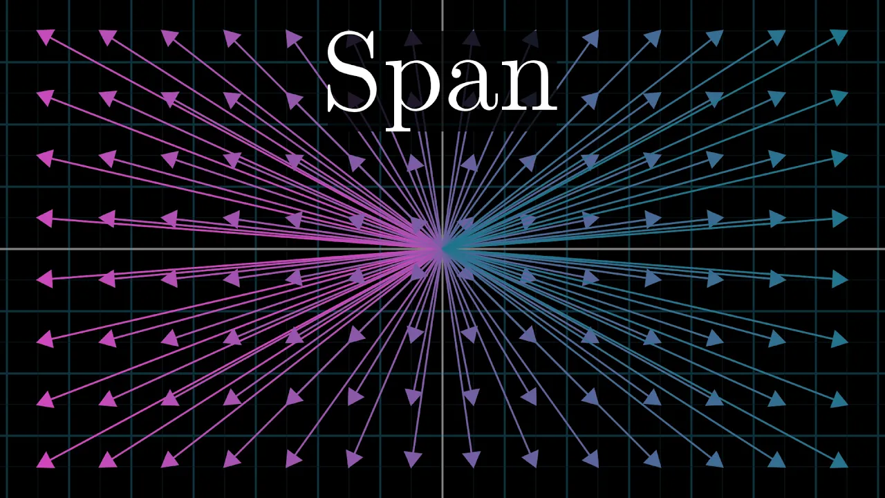
Why this video

This video provides an elegant visual model of how coordinate systems are built. To transition into tensor calculus, you must move away from treating vectors as "arrows in a fixed grid" and start seeing them as linear combinations of arbitrary, dynamic basis vectors.

Knowledge Checkpoint

• Define what a "basis" is in a vector space.
• Explain how scaling basis vectors changes the numerical coordinates of a vector.
• Visualize how linear combinations span space.

---

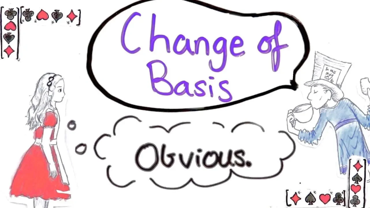
Why this video

Tensors are mathematically defined by how their components transform under a change of basis. This video explains the transformation formulas and translates the intuitive geometry of changing basis sets into concrete matrix algebra.

Knowledge Checkpoint

• Construct a change-of-basis matrix to translate vectors between two coordinate systems.
• Differentiate between the transformation of basis vectors and the transformation of vector components.
• Explain how a vector remains invariant even when its components change.

---

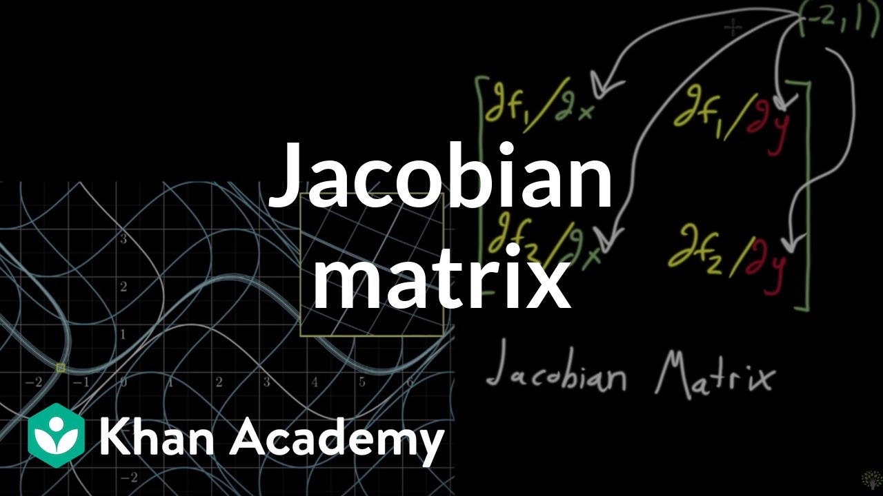
Why this video

In curved spaces, transformations are rarely linear globally. The Jacobian matrix is the key tool that locally linearizes non-linear coordinate mappings (like Cartesian to polar/spherical coordinates), serving as the foundational tool for coordinate transformations in differential geometry.

Knowledge Checkpoint

• Calculate the Jacobian matrix for a multi-variable transformation.
• Explain the geometric meaning of the Jacobian determinant as a local area scaling factor.
• Interpret the Jacobian as a linear approximation of a non-linear function near a point.

---

Why this video

This video provides an intuitive and physical understanding of the gradient ($\nabla f$), divergence ($\nabla \cdot \mathbf{F}$), and curl ($\nabla \times \mathbf{F}$). Seeing these operators in flat spaces helps you identify why standard partial derivatives fail on curved manifolds and why we need covariant derivatives later.

Knowledge Checkpoint

• Describe the physical meaning of gradient, divergence, and curl.
• Explain how the Del operator ($\nabla$) acts as a symbolic vector.
• Understand how these operators are calculated in standard Euclidean coordinates.

---

Module 2: Covectors, Dual Spaces, and Tensor Basics

This module transitions you from classic vector spaces to dual spaces. You will discover covectors (one-forms), understand how they differ geometrically from standard vectors, and explore how covariant and contravariant components transform under coordinate changes.

Recommended Videos

Why this video

This is a highly popular, clear, and conceptual introduction to tensors. It bridges the gap between simple scalars/vectors and higher-rank structures, defining tensors by how their components respond to spatial transformations.

Knowledge Checkpoint

• Define a tensor's rank and explain what a rank-0, rank-1, and rank-2 tensor represent.
• Explain why a vector is a rank-1 tensor and a scalar is a rank-0 tensor.
• Describe how tensor components change when coordinate axes are scaled.

---

Why this video

Covectors (or dual vectors) are difficult to grasp conceptually. This video visualizes covectors not as arrows, but as oriented parallel planes or contour stacks. This visualization makes the contraction between vectors and covectors intuitive.

Knowledge Checkpoint

• Contrast the visual representation of a vector (an arrow) with a covector (contour lines).
• Explain how a covector acts as a linear map that transforms a vector into a scalar.
• Describe the relationship between a vector space $V$ and its dual space $V^*$.

---

Why this video

This video clarifies the transformation differences between contravariant components (index upstairs: $V^i$) and covariant components (index downstairs: $U_i$). It explains how contravariant components scale opposite to the basis vectors, while covariant components scale alongside them.

Knowledge Checkpoint

• Write down the coordinate transformation equations for contravariant vector components.
• Write down the coordinate transformation equations for covariant vector components.
• Explain why the gradient of a scalar function naturally transforms as a covariant vector (covector).

---

Module 3: The Metric Tensor and Index Gymnastics

This module introduces the metric tensor, the mathematical tool used to measure distances, angles, and volumes in curved spaces. You will also learn the rules of the Einstein summation convention and how to raise and lower indices.

Recommended Videos

Why this video

Tensor calculus equations can become cluttered with summation signs ($\sum$). This video explains the Einstein summation convention, where any repeated index in a term automatically implies summation over all possible values of that index.

Knowledge Checkpoint

• Identify "dummy indices" and "free indices" in a tensor equation.
• Expand an expression written in Einstein notation into an explicit sum.
• Recognize invalid expressions that violate the summation rules.

---

Why this video

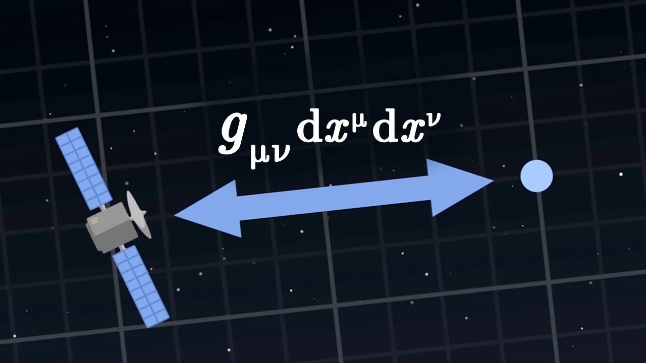
An exceptional visual and mathematical guide to the metric tensor ($g_{\mu\nu}$). It illustrates how the metric generalizes the Pythagorean theorem to arbitrary curved spaces, allowing you to calculate the length of an infinitesimal interval $ds^2$.

Knowledge Checkpoint

• Define the metric tensor as an inner product of basis vectors: $g_{ij} = \mathbf{e}_i \cdot \mathbf{e}_j$.
• Write down the line element $ds^2$ using the metric tensor and differential coordinates.
• Explain how the metric tensor changes when transitioning from flat Minkowski space to a curved geometry.

---

Why this video

This video bridges a common gap in tensor learning: the mechanics of "index gymnastics." It explains how to use the metric tensor $g_{ij}$ and its inverse $g^{ij}$ to convert contravariant components into covariant components and vice versa.

Knowledge Checkpoint

• Lower a contravariant index using the metric tensor: $V_i = g_{ij} V^j$.
• Raise a covariant index using the inverse metric tensor: $V^i = g^{ij} V_j$.
• Explain why the metric tensor and its inverse contracted together yield the Kronecker delta: $g_{ik}g^{kj} = \delta_i^j$.

---

Gap-Filling Tutorial: Index Gymnastics

Algebraic Verification Exercise:
Let the metric of a 2D polar coordinate system $(r, \theta)$ be represented as: $g_{ij} = \begin{pmatrix} 1 & 0 \\ 0 & r^2 \end{pmatrix}$

1. Find the inverse metric $g^{ij}$: $g^{ij} = \begin{pmatrix} 1 & 0 \\ 0 & \frac{1}{r^2} \end{pmatrix}$
2. Let a contravariant vector field be $V^i = (v^r, v^\theta) = (2, 3)$.
3. Lower the index to find the covariant components $V_i$: $V_r = g_{rr} V^r + g_{r\theta} V^\theta = 1(2) + 0(3) = 2$ $V_\theta = g_{\theta r} V^r + g_{\theta\theta} V^\theta = 0(2) + r^2(3) = 3r^2$ $V_i = (2, 3r^2)$

---

Module 4: Covariant Derivatives and Christoffel Symbols

In flat spaces, basis vectors are constant everywhere. In curved spaces, basis vectors change from point to point. This module covers the covariant derivative, parallel transport, and Christoffel symbols (connection coefficients), which correct for this changing basis during differentiation.

Recommended Videos

Why this video

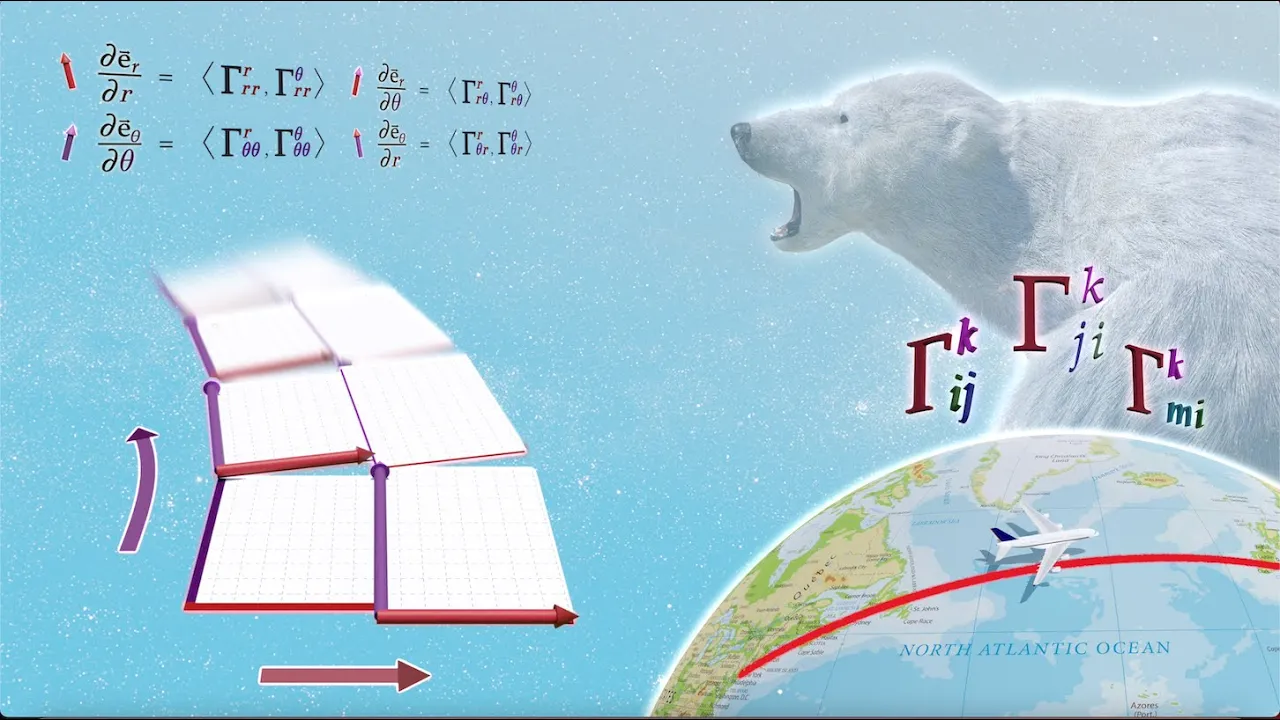
This video explains why ordinary partial derivatives fail in curvilinear coordinates. It introduces Christoffel symbols as geometric correction terms that measure how basis vectors rotate and stretch across space.

Knowledge Checkpoint

• Explain why $\partial_j V^i$ does not transform as a tensor.
• Describe the physical/geometric meaning of the Christoffel symbols $\Gamma^i_{jk}$.
• Visualize how curvilinear grids (like polar coordinates) make coordinate lines curve even in flat space.

---

Why this video

This video provides the explicit algebraic derivations for Christoffel symbols. It derives them using the metric compatibility condition $\nabla_k g_{ij} = 0$, leading to the standard formula in terms of partial derivatives of the metric.

Knowledge Checkpoint

• Write down the general formula for computing the Christoffel symbols of the second kind: $\Gamma^k_{ij} = \frac{1}{2} g^{kl} \left( \partial_i g_{jl} + \partial_j g_{il} - \partial_l g_{ij} \right)$
• Compute Christoffel symbol values from a given metric tensor.
• Understand the symmetry property of Christoffel symbols in a torsion-free space ($\Gamma^k_{ij} = \Gamma^k_{ji}$).

---

Why this video

This video introduces parallel transport and the covariant derivative ($\nabla_\mu V^\nu$). It explains how to compare vectors at different points on a curved manifold by transporting them along a curve while keeping them parallel to themselves.

Knowledge Checkpoint

• Write down the covariant derivative formula for a contravariant vector: $\nabla_k V^i = \partial_k V^i + \Gamma^i_{jk} V^j$.
• Write down the covariant derivative formula for a covariant vector: $\nabla_k V_i = \partial_k V_i - \Gamma^j_{ki} V_j$.
• Explain parallel transport using the covariant derivative.

---

Step-by-Step Calculation: Christoffel Symbols on a 2D Sphere

To compute the Christoffel symbols for a sphere of radius $R$ with metric $ds^2 = R^2 d\theta^2 + R^2 \sin^2\theta d\phi^2$:

Here, $g_{\theta\theta} = R^2$, $g_{\phi\phi} = R^2 \sin^2\theta$, and $g^{\theta\theta} = \frac{1}{R^2}$, $g^{\phi\phi} = \frac{1}{R^2 \sin^2\theta}$.

Let's calculate $\Gamma^\theta_{\phi\phi}$: $\Gamma^\theta_{\phi\phi} = \frac{1}{2} g^{\theta\theta} \left( \partial_\phi g_{\phi\theta} + \partial_\phi g_{\phi\theta} - \partial_\theta g_{\phi\phi} \right)$ Since $g_{\phi\theta} = 0$: $\Gamma^\theta_{\phi\phi} = \frac{1}{2} \left(\frac{1}{R^2}\right) \left( 0 + 0 - \frac{\partial}{\partial\theta} (R^2 \sin^2\theta) \right) = \frac{1}{2R^2} \left( -2R^2 \sin\theta \cos\theta \right) = -\sin\theta \cos\theta$

---

Module 5: The Riemann Curvature Tensor and General Relativity

This module marks the culmination of the curriculum. You will explore how the Riemann curvature tensor measures spacetime curvature, derive the geodesic equation, and study its application in Einstein's field equations.

Recommended Videos

Why this video

Geodesics are the paths of shortest distance on curved surfaces, generalising "straight lines." This video derives the geodesic equation from the calculus of variations by minimizing the arc length functional, addressing a common gap in differential geometry courses.

Knowledge Checkpoint

• Write down the geodesic equation: $\frac{d^2 x^k}{d\lambda^2} + \Gamma^k_{ij} \frac{dx^i}{d\lambda} \frac{dx^j}{d\lambda} = 0$
• Explain how the geodesic equation describes motion without external forces in general relativity.
• Relate the second derivative term (acceleration) to the Christoffel symbols (geometric gravity).

---

Why this video

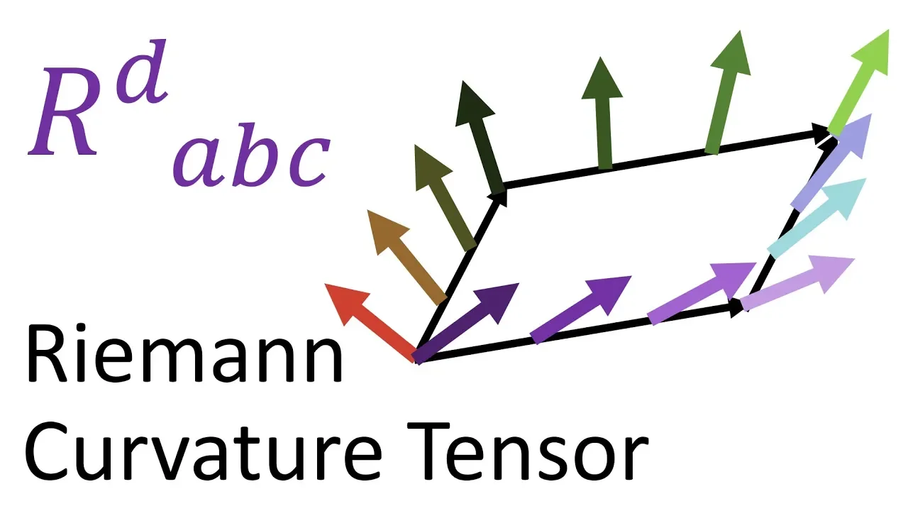
This video explains the geometric meaning of the Riemann curvature tensor using holonomy and geodesic deviation. You will see how parallel transporting a vector around a closed loop in curved space results in a net rotation, and how the Riemann tensor measures this mismatch.

Knowledge Checkpoint

• Explain how non-commuting covariant derivatives reveal curvature: $(\nabla_i \nabla_j - \nabla_j \nabla_i) V^k = R^k_{lij} V^l$.
• Define "holonomy" and explain its relationship to curvature.
• Describe the concept of geodesic deviation (how parallel paths diverge or converge).

---

Why this video

This university-level lecture provides a detailed mathematical calculation of the Riemann curvature tensor from start to finish. It is ideal for filling analytical gaps, demonstrating exactly how to write out and sum all the index terms.

Knowledge Checkpoint

• State the coordinate formula for the Riemann tensor: $R^a_{\ bcd} = \partial_c \Gamma^a_{bd} - \partial_d \Gamma^a_{bc} + \Gamma^a_{ce}\Gamma^e_{bd} - \Gamma^a_{de}\Gamma^e_{bc}$
• Explain the algebraic symmetries of the Riemann tensor (antisymmetry on final two indices, cyclic Bianchi identity).
• Trace how the Ricci tensor ($R_{ab} = R^c_{\ acb}$) and Ricci scalar ($R = g^{ab}R_{ab}$) are obtained through index contraction.

---

Why this video

This video brings together all the concepts covered in this curriculum (metrics, connections, and curvature) to construct Einstein's Field Equations. It shows how the geometry of spacetime (Einstein tensor $G_{\mu\nu}$) is coupled to mass-energy density (energy-momentum tensor $T_{\mu\nu}$).

Knowledge Checkpoint

• Write down the Einstein Field Equations: $R_{\mu\nu} - \frac{1}{2}g_{\mu\nu}R = \frac{8\pi G}{c^4} T_{\mu\nu}$
• Identify which parts of the equation represent geometry versus energy-matter content.
• Explain how the metric tensor acts as the gravitational potential in relativistic physics.

---

Course Map

---

Key People Index

• Bernhard Riemann (1826–1866): Developed the foundations of elliptic and intrinsic geometry, proving that spaces can be curved intrinsically without needing to be embedded in higher-dimensional space.
• Albert Einstein (1879–1955): Utilized tensor calculus to construct General Relativity, formulating gravity not as an attractive force, but as the geometric curvature of four-dimensional spacetime.
• Elwin Bruno Christoffel (1829–1900): Developed the connection coefficients (Christoffel symbols) that describe how basis vectors change dynamically across a curved manifold.
• Gregorio Ricci-Curbastro (1853–1925) & Tullio Levi-Civita (1873–1941): Developed absolute differential calculus (now known as tensor calculus), providing the mathematical framework that Einstein eventually used to formulate his equations.

---

Final Self-Assessment

Complete this comprehensive self-assessment to test your understanding of the curriculum.

• I can write the coordinate transformation equations for any arbitrary rank-2 tensor $T^i_{\ j}$.
• I can explain the geometric difference between a vector and a covector.
• I can write out the Einstein summation convention expansion for $A_i B^i$ in a 4-dimensional space.
• I can calculate the metric tensor $g_{ij}$ and its inverse $g^{ij}$ for any given 2D surface (e.g., a cylinder, cone, or sphere).
• I can raise and lower indices in complex tensor equations using the metric tensor.
• I can explain why the ordinary partial derivative of a vector does not yield a tensor under general coordinate changes.
• I can write down the geodesic equation and explain the physical meaning of each term.
• I can compute all non-zero Christoffel symbols for simple, diagonal 2D metric profiles.
• I can write down the algebraic formula for the Riemann curvature tensor $R^a_{\ bcd}$ and explain its relationship to parallel transporting vectors around loops.
• I can contract the Riemann curvature tensor to obtain the Ricci tensor and the Ricci scalar.
• I can write out the full Einstein field equations and identify the terms representing spacetime curvature and matter-energy.