
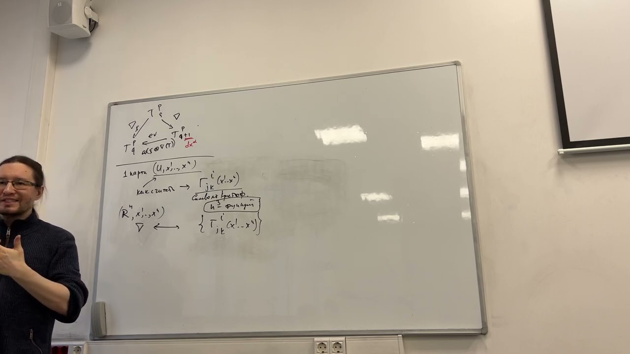


![[확률론과 미분기하는 미적분학 이다 2기] Connection and Christoffel symbols, History of Relativity theory](https://i.ytimg.com/vi/64D2EOQxzHE/maxresdefault.jpg)

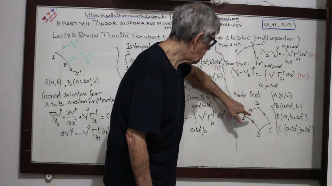
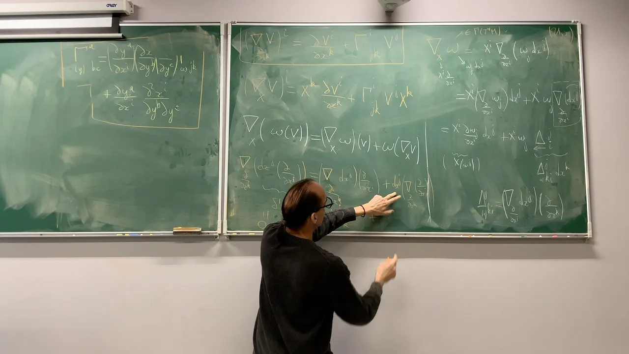

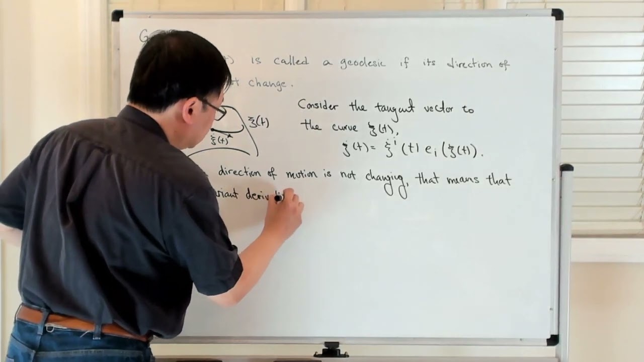



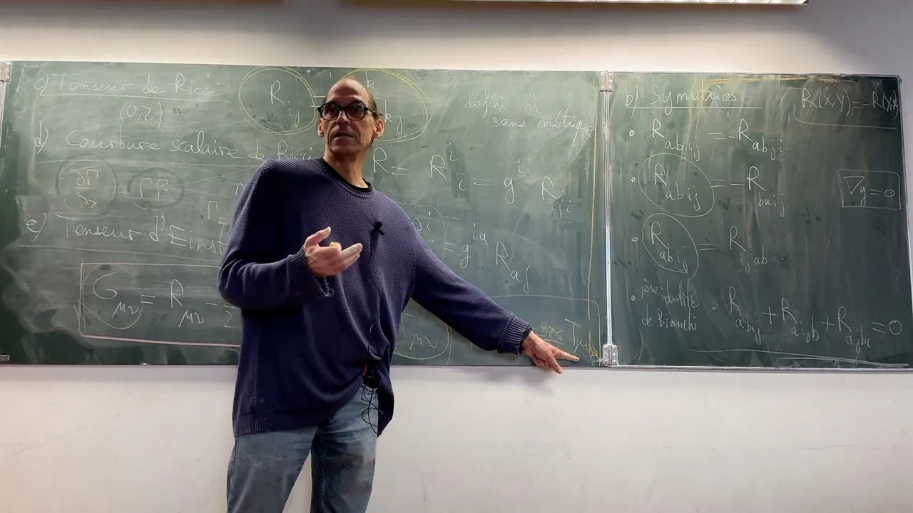
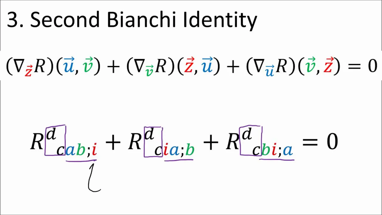
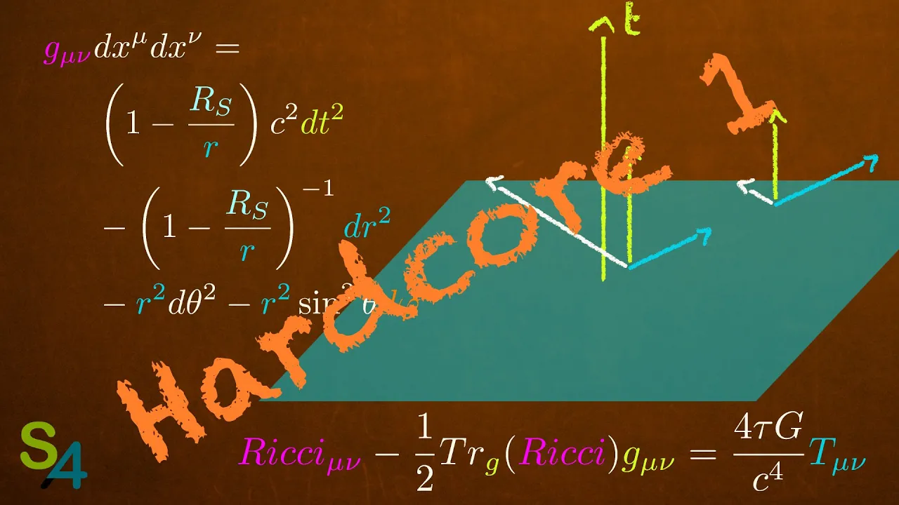


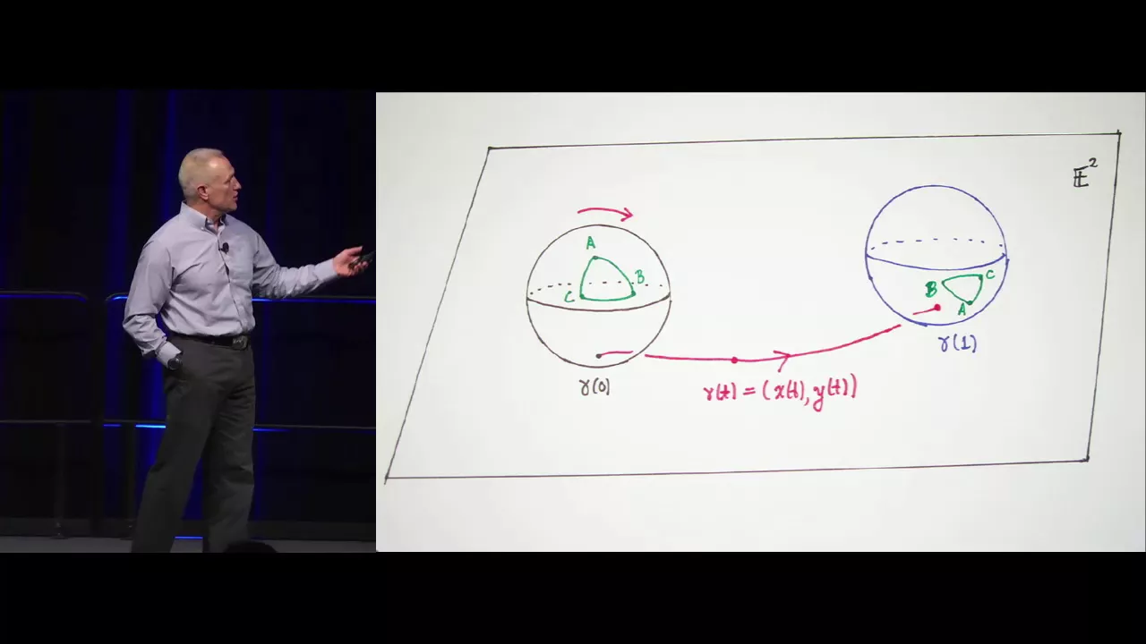


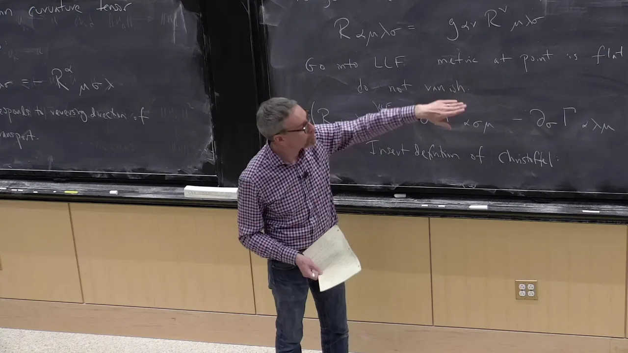


The Riemann curvature tensor detects whether a space is curved or flat by measuring the failure of parallel transport around a closed loop (holonomy) or the acceleration of nearby geodesics (geodesic deviation); unlike connection coefficients which can be zero in any coordinate system at a point, the Riemann tensor provides an invariant geometric measure of curvature through the formula R(U,V)W = ∇_U∇_VW - ∇_V∇_UW - ∇_[U,V]W, where the Lie bracket term accounts for non-commuting vector fields.
Riemann Curvature Tensor: Geometric Meaning in Tensor Calculus
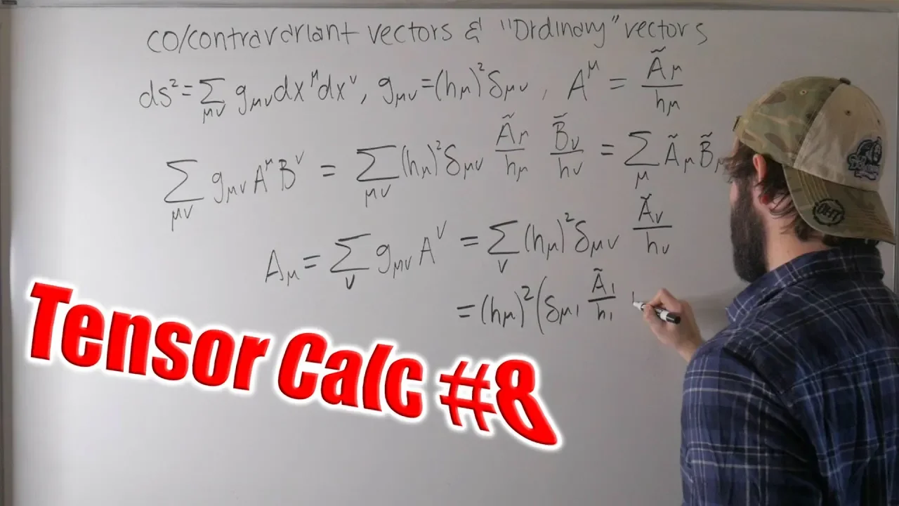
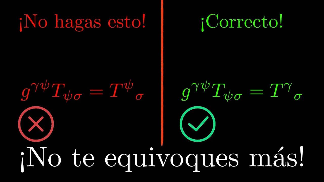
Added:Fundamentals of tensor calculus, including Einstein summation convention, covariant and contravariant indices, and the metric tensor.
The concept of the covariant derivative and Christoffel symbols (affine connections) on differentiable manifolds.
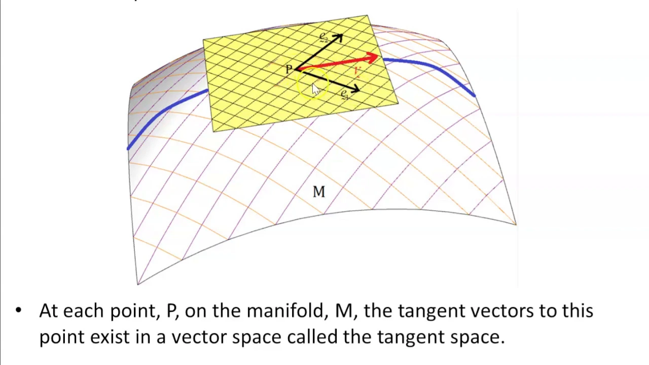
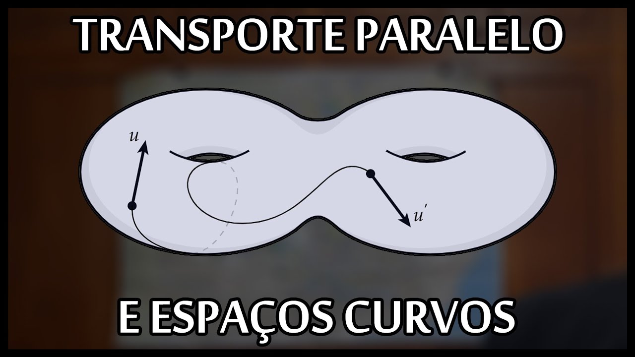
Parallel transport of vectors along curves, which is fundamental to understanding how vectors change in curved spaces.
The definition and formulation of geodesics as the generalization of straight lines to curved manifolds.
Contractions of the Riemann tensor to define the Ricci curvature tensor and the Ricci scalar (curvature scalar).
Einstein's Field Equations in General Relativity, which relate the curvature of spacetime (using the Riemann/Ricci tensors) to energy and momentum.
Advanced study of Holonomy Groups and their role in the classification of Riemannian manifolds (e.g., Calabi-Yau manifolds in string theory).
Physical applications of the geodesic deviation equation, specifically in modeling tidal forces and analyzing gravitational waves.
131.7K views2.8Klikes29:13Original Release: 2019-06-16
in this video I'm going to talk about the Riemann curvature tensor which is a mathematical tool that helps us figure out if a space is curved or flat I'm expecting you already understand the covariant derivative and the Li bracket if you don't know what those are please check the description for links to my previous videos on those topics I'm going to derive the abstract formula for the Riemann tensor and give an explanation of its geometric meaning if you want to learn about the Riemann tensor components and its symmetries you'll have to look at the next video in this series and just a reminder I'll be using any of these symbols to denote basis vectors in this video these all mean the same thing and remember the covariant derivative of a vector in a given Direction is given by this formula here where these gammas are the connection coefficients and while there are many possible definitions for the connection coefficients the most common definition you'll see is the levee to Vedic connection which I covered in video xx so the main question we want to answer is how can we tell if a space is curved or flat and you might think that this is an easy question that we can answer just by using our eyes clearly a sphere is curved and clearly a plane is flat but a lot of the time in math we don't have the luxury of visualizing a space with a picture instead all we have to look at our coordinate system and a metric tensor matrix which measures lengths and angles in the coordinate system so what we need is some sort of mathematical procedure for using the metric tensor to determine whether a space is curved or flat we can also use the connection coefficients in this procedure because the connection coefficients are calculated using the derivatives of the metric tensor to get an idea of what flat space looks like let's take a look at the 2d plane with Cartesian coordinates in this coordinate system the metric tensor is the identity matrix and all the connection coefficients are 0 according to the geodesic equation when the connection coefficients are 0 the geodesic curves just end up being straight lines which is exactly what we would expect for flat space so this be our first attempt at a definition for flat space when all the connection coefficients are 0 the space is flat this gives us geodesics which are straight lines so the space would appear to be flat however it's not that easy we know that 2d polar coordinates also describe flat space but the metric tensor is not the identity matrix and the connection coefficients are not all 0 however we can transform polar coordinates into Cartesian coordinates using the Jacobian to transform the basis vectors the metric tensor and the connection coefficients so attempt number two at defining flat space is to say that a space is flat when we can make the connection coefficients all equal to 0 using a change of coordinates under this definition the 2d plane would be flat even if we're using a curvilinear coordinate system like polar coordinates however this definition isn't good enough either if we take the sphere which we know is a curved surface and look at the equator where the first coordinate in the standard coordinate system is equal to PI over 2 we find that on the equator the connection coefficients are all equal to 0 and of course since the equator is an arbitrary circle we can always change coordinates to make any point lie on the equator of the coordinate system if we choose so it turns out that in curved spaces sometimes called manifolds we can always find a special coordinate system called the riemann normal coordinates or the local inertial frame where the metric tensor is the identity matrix and the connection coefficients are all 0 for a specific point this won't be true everywhere in the space but it will be true for that specific point so the connection coefficients being 0 isn't good enough to detect whether a space is curved at a given point because we can always pick a coordinate system that makes the connection coefficients go to 0 so to curvature in a space we need a new tool and that new tool is the Riemann curvature tensor R which is a once contravariant three times covariant tensor and there are two ways we can use the Riemann curvature tensor to detect curvature the first is detecting what's called Helana me and the second is detecting geodesic deviation in this video I'm going to focus on the Helana me definition of the Riemann curvature tensor if you recall in video 18 I introduced the idea of parallel transport of vectors which keeps a vector as constant as possible as we move it step by step around on a surface so if a person at the North Pole was carrying a spear or a harpoon and they started walking forward keeping the spear as straight as possible when they got to the equator the spear would be pointing in this direction and this is just like parallel transporting a vector along a curve and if we keep parallel transporting the vector along the equator we'd get this and if we parallel transported it backward up to the North Pole again we'd get this so you'll notice that after parallel transporting the vector around in a loop the vector has twisted around a bit and points in a different direction compared to where it started and this is what Helana me refers to Helana me is the twisting of a vector when we transport it around in a loop and this is one way we can detect if a space is curved if we have a flat space like the surface of a table and we move a vector around in a loop keeping it as straight as possible the vector will be pointing in the same direction at the start of the loop and at the end of the loop however if we're in some other space and we move the vector around in a loop and it's pointing in a different direction compared to the starting direction the only possible explanation is that the space were in is curved for example the curved surface of the sphere so let's use this idea to determine a formula for the Riemann curvature tensor let's take two vector fields U and V and you them to create a small parallelogram we're going to assume that the Li bracket of U and B is 0 so the vectors will close together properly without a gap as we learned in video 21 I'm going to label the four corners of this parallelogram by the points 0 0 R 0 RS and 0s next we're going to take this vector W and parallel transport it around the parallelogram so we'll say that the linear map a parallel transports W from this point along the vector u to this point and we'll say that the linear map be parallel transports W along V from this point to this point linear map C takes W from this point to this point and D takes W from this point to this point so to parallel transport W around the parallelogram we apply a then B then C then D and to compare this to the original vector we subtracted from W so remember in flat space the vectors should point in the same direction at the beginning and at the end so in flat space this difference should be 0 if this difference between the starting and ending vectors is nonzero that tells us that the space is curved now the difference between the W vector and it's parallel transported version dcba W will tell us about the curvature of the space across this parallelogram but we're generally going to be interested about the curvature information at a single point such as the point 0 0 here so to get the curvature information at this point we take the limit as the R and s variables go to 0 we also divide by the product of R and s to make the answer independent of the area of the parallelogram so this limiting process will tell us how much the vector W changes when it is parallel transport around a very very small parallelogram near the point zero zero and we are going to denote this formula by R of U and V acting on W here R is the Riemann curvature tensor and U and V are the vectors that make up the parallelogram R of U and V is an operator which acts on the vector W and outputs the change vector after it is parallel transported around a small parallelogram so we can think of the Riemann curvature tensor as taking three vector inputs two vectors defining the parallelogram and a starting input vector and it outputs this change vector here after W is parallel transported around the parallelogram so let's see if we can get a formula for R of U and V acting on W first I'm going to multiply this W vector by DC C inverse D inverse these four operators multiplied together are equal to the identity matrix so it doesn't change the vector W in any way next I'm going to factor out DC from both terms now I'm going to take this term inside the brackets and rewrite it I'm going to add and subtract C inverse times W as I've done here then I'm going to add and subtract BW and then I will add and subtract W so since all of these terms will cancel with each other this is the same thing as adding 0 so the final result won't change I'm also going to factor out negative 1 from this set of terms and bring a minus sign outside the parentheses this will flip all the signs inside the brackets next I'll factor out C inverse from here and factor B from here now some of you may have noticed that there's a bit of a problem here this formula has a bunch of subtractions in it that don't really make sense if we got a W - W the W vector is located here at the point 0 0 and the a W vector is located here at the point R 0 the vectors live in different tangent spaces and we can't subtract them this would be like trying to subtract two vectors on different points of a sphere it just doesn't make sense and right now the subtractions in this formula don't make sense either to fix this we can take the vector W and extend it into a full vector field around the parallelogram the vector field can be any vector field we want as long as it agrees with the original W vector at the origin and changes smoothly from point to point the exact details of how we create this vector field don't actually matter we'll find that the final result of our formula doesn't actually depend on the vector field at all what's important is that we can now take the parallel transported vectors of the initial W vector and compare them with the vectors in the W vector field at the same point this means that the subtraction a W minus W now makes sense if we think of W as a vector field and not just as a single vector at the point 0 0 ok so looking at this limit the terms inside the brackets are equal to this and we can distribute the 1 over R times s to the various terms inside the brackets to get this but notice that when we take the limit as R goes to 0 that means that the vector paths for a and C go to 0 and when we take the limit of the difference between W and W parallel transported along the a operator all divided by R which is proportional to the length of the vector that's the same thing as the covariant derivative along u because the a operation makes us travel in the U direction and measuring how much the W vector field deviates away from parallel transport is the same thing as taking the covariant derivative and the same thing is true with the see inverse operator since C inverse points in the opposite direction of C meaning at points in the U Direction this becomes the covariant derivative along U as well and when we take the limit as s goes to 0 the vector paths for B and D go to 0 and the limit of this difference and this difference is just the covariant derivative along V since both B and D inverse point in the V direction so we have this and rearranging the terms we get these two differences and again taking the limits as R and s go to 0 this becomes the covariant derivative along U and this becomes the covariant derivative along V and finally as R and s go to 0 these D and C operators just both become an identity matrix since parallel transporting along a curve of 0 length means the vector doesn't change at all so these operators just become the identity matrix in the limit so the formula for parallel transporting the vector W along a parallelogram is right here it's the difference of these two covariant derivatives along U and be applied to W however recall that we started with the assumption that the Li bracket of U and B is 0 this formula works fine when the Li bracket of U and B is 0 however when the Lee bracket is nonzero we actually need this extra term on the formula here subtracting the covariant derivative of W in the direction of the Li bracket of U and V while researching this video I tried looking at a bunch of different sources to try and understand why this third term is necessary unfortunately I wasn't able to find any explanations that really convinced me however I can give you two reasons that are at least somewhat convincing reason number one is that this third term takes care of the gap in the parallelogram when the Leigh Brackett is non-0 reason number two is that this third term is required to make our a true tensor in other words it's needed to make sure our is a multi linear map reason number one comes from section eleven point four of the gravitation textbook by Misner thorne and wheeler if you watched video 21 you'll know that the flow curves along two vector fields U and V don't always form a nice parallelogram the gap that results here is given by the lee bracket of U and B the gravitation textbook makes the claim without a convincing formal proof that this third term in the formula is what's required to parallel transport a vector around all five sides of this loop including the lee bracket part again I can't prove that this is true but given that the Lee bracket appears in both places it seems possible reason number two is that this third term is required to make our attend sir in other words it's needed to make sure that the UV and W input slots are all linear and recall that a functions input is linear when we can scale the input or scale the output and get the same result and when we add inputs or add outputs we get the same result now the reason that we want R to be a tensor is because tensors are geometrical objects that everyone can agree on for example everyone can agree this vector is an arrow that's pointing towards the square the components of the vector might look different in different coordinate systems but everyone will agree on geometrical facts like the vectors length and direction the Riemann tensor should be the same way if we parallel transport W around the parallelogram made up by the U and V vectors the result should be something that everyone agrees on it shouldn't depend on the coordinates so if R is a tensor then we should be able to take the U input vector and expand it as a linear combination and pull the components and the summation outside of the function the same would apply to the V and W inputs if R is a multi linear function that means that to compute R of U and V acting on w we can pull all the vector components out in front and we only need to compute how our acts on a set of basis vectors in order to get the final result so I'll go ahead and prove that this formula is linear in each of you V and W to start I'll mention that the Li bracket is not linear in its inputs the Li bracket of are scaled by a and s is not the same thing as the Li bracket of our NS scaled by a this is because when we write out the formula for the Lee bracket the scalar a ends up inside this derivative here so we need to apply a product rule to get two terms then we can factor out a from these two terms and get this and this is just the definition of the Li bracket of r and s so you can see that the Li bracket inputs are not linear because scaling the input and scaling the output are not the same thing we get this extra term left over with that in mind let's prove that the Riemann tensor is linear in the U input so we can expand U as a linear combination and if we recall this Li bracket formula we derived on the last slide we can apply it to this Li bracket up here to get this and since the direction vector input of the covariant derivative is linear we can pull the UI components out in front like this so here we have the covariant derivative of a product so we use the product rule to expand this into two terms and recall the covariant derivative of a scalar is just the ordinary derivative so we can turn this into an ordinary derivative this cancels with this and we can factor out the UI out of all the remaining terms and this is just the Riemann tensor of the e aí basis vector and V and W so we've shown that the Riemann tensor is linear for the you input the proof that the V input is linear is almost the exact same except the terms appear in a different order so I'm not going to bother proving it next I'll prove that the W input slot of the Riemann tensor is linear to begin I'm going to look at the first two terms only with the W vector expanded in a linear combination taking the inner covariant derivative we use product rule in each term to give us a total of four terms and taking the outer covariant derivative we use product rule again giving us a total of eight terms thankfully this cancels with this and this cancels with this so we have four terms remaining so the first two terms in the Riemann tensor formula expand to these four terms and looking at the third term with the Li bracket if we use the product rule here we'll get another two terms one with the derivative of the components and one with the derivative of the basis vector now I'd like to point out that for scalars taking the covariant derivative of V than you minus the covariant derivative of U then V is the same thing as taking the covariant derivative of the Lee bracket of U and V this is because for scalars the covariant derivative is just the ordinary derivative so both sides just end up being the commutator of U and V this means that these two terms cancel with this term since we're taking the covariant derivative of the components of W which are scalars so ignoring those we have three terms left over and factoring out the W components we see that this is just the definition of the Riemann tensor acting on the basis vectors so the Riemann tensor is indeed linear in the W input slot okay so we've proven that the Riemann curvature tensor is linear in all of its inputs and that means that to compute the result for any combination of input vectors we really just need to know how it acts on the basis vectors and this here actually ends up being the components of the Riemann tensor but I'm going to cover that in the next video to summarize this video we learned about the Riemann normal coordinates or local inertial frame which is a coordinate system at a point P where the metric tensor is the identity matrix and all the connection coefficients are 0 because we can always find a coordinate system where this is true at a given point the connection coefficients being zero is not enough to detect whether or not a space is flat instead we use the Riemann curvature tensor given by this formula here this represents taking a parallelogram formed by the vector field to U and V and parallel transporting a vector W around it the output is the difference between the original W vector and it's parallel transported version if this difference vector is zero we know the space is flat if it's nonzero the space is curved we also showed how the Riemann curvature tensor is linear in all of its inputs the last thing I'll talk about is another geometric interpretation of the Riemann tensor which is geodesic deviation geodesic deviation is another way to tell if a space is curved or flat imagine that we're in flat space and we pick some point P if we start walking outward from this point we'd trace out a geodesic path which would be a straight line in flat space and if we walked outward at a slightly different angle we'd get this geodesic and with other angles we'd get other geodesics on the other hand if we're on a curved space like the sphere and we picked a point say the North Pole and created paths walking outward from this point these geodesic paths would look like this now in flat space the separation between these geodesics changes at a constant rate in other words if we looked at these separations between these geodesics one second into their journeys and we compared that to the seperation to seconds along each of the journeys the separations at the two second mark would be twice as big as the separations at the one second mark in other words if we drew a separation vector s between two of the paths at various points this separation vector will be changing in size and the rate of change or the derivative of this vector along a geodesic would be a constant number since the rate of growth of the vector is constant this means that the second derivative would be zero now on the other hand the separation between geodesics on the sphere does not change at a constant rate the curves are actually accelerating away from each other and then accelerate toward each other once they cross the equator so in this case the second covariant derivative of the separation vector is nonzero because there is acceleration going on because the geodesics are either accelerating apart or accelerating toward each other so this is another way to tell if a space is flat or curved by looking at whether or not the separation vector between geodesics is accelerating so if we have a family of geodesics coming out of a point P we can describe the tension vectors along these geodesics by the vector field V so since the V vectors are tangent to the geodesics they're a bit like velocity vectors along the geodesics and we can describe the separation between these geodesics at various points in time by these separation curves you can think of this curve as marking the point where we've been traveling along the geodesics for one second this curve marks the two second point and this curve marks the three second point the tangent vectors along these separation curves will be given by the vector field S these S vectors would be the separation vectors between the geodesics now we want to compute the geodesic deviation which is the second rate of change of the separation vector s as we travel along the geodesics in the direction of B now we're going to assume that we're in a space where the connection is torsion free in other words the difference between these two covariant derivatives is equal to the Li bracket of the ns but since the V and s vector field flow curves form a grid nice closed parallelograms there Li bracket is zero so bringing this to the other side we find that we can swap the order of these two vectors in the covariant derivative if the connection is torsion free alright so given that the curves tangent to V are geodesics this means that the covariant derivative of V along itself is zero remember this was one of the definitions of geodesics we gave in video 19 curves that are parallel transported along themselves and we can of course take the covariant derivative with respect to s on both sides and the right hand side stays zero now we're going to take this formula and add and subtract this term here now this subtraction is equal to the Riemann tensor of s and V applied to V there are only two terms here but remember since the Li bracket of s and V is zero we can ignore the third term of the Riemann tensor formula that involves the Li bracket also here we're going to swap the V and s vectors because of the torsion free property so we've determined that the geodesic deviation or the second derivative of the separation vector along the geodesics is equal to this negative Riemann tensor term and of course if the Riemann tensor is zero everywhere this must mean the geodesic deviation is also zero so these space is flat so this is another interpretation of the Riemann tensor for determining if a space is curved or flat if the Riemann tensor is zero we know the second derivative of the separation vector is also zero and that means that the separation vector is changing at a constant rate in other words the geodesics are not accelerating away or toward each other and we can conclude we're in a flat space on the other hand if the geodesic deviation is non zero that means that the geodesics either accelerating toward or away from each other and that means that the space is curved in the next video we'll compute the Riemann tensor components for the sphere and also look at these symmetries of the Riemann tensor if you like my videos please check the links in the description and consider supporting me
Up Next

62:48
Riemann Tensor: Newtonian Limit, 2-Sphere, Accelerating Coordinates
@centrumfizykiteoretycznejp6497
180 views•2024-05-07

4:43
Elliptic Curve Cryptography Explained: ECC, ECDSA, ECDH
@PracticalNetworking
28.5K views•2024-10-21
14:07
Understanding Covectors in Tensor Algebra: Linear Functions Explained
@eigenchris
308.8K views•2017-12-15

6:00
The Mathematical Impossibility of Accurate World Maps
@Vox
23.3M views•2016-12-02
Related Study Plans & Knowledge Roadmaps
Structured learning paths in Mathematics
mathematics
Tensor Calculus: Vectors to Riemann Curvature
01Mathematical Foundations: Linear Algebra & Calculus
02Covectors, Dual Spaces, and Tensor Basics
03The Metric Tensor and Index Gymnastics
+ 2 more learning modules
40h5 modules
Explore Roadmap
mathematics
Gödel's Incompleteness: Logic, Proofs & Limits
01Introduction to Formal Systems & Hilbert's Dream
02Set Theory, Cardinality, and Cantor's Diagonal Argument
03Arithmetization and Gödel Numbering
+ 2 more learning modules
14h5 modules
Explore Roadmap
mathematics
Galois Theory: Fields, Groups & Solvability
01Foundations of Abstract Algebra: Groups & Fields
02Polynomials & Field Extensions
03Splitting Fields & Symmetries
+ 2 more learning modules
24h5 modules
Explore Roadmap
mathematics
Non-Euclidean Geometry: Models & Geodesics
01Euclid's Fifth Postulate and the Birth of New Geometries
02Hyperbolic Space and the Poincaré Disk Model
03Geodesics: Defining Straight Lines in Curved Spaces
+ 2 more learning modules
15h5 modules
Explore Roadmap