
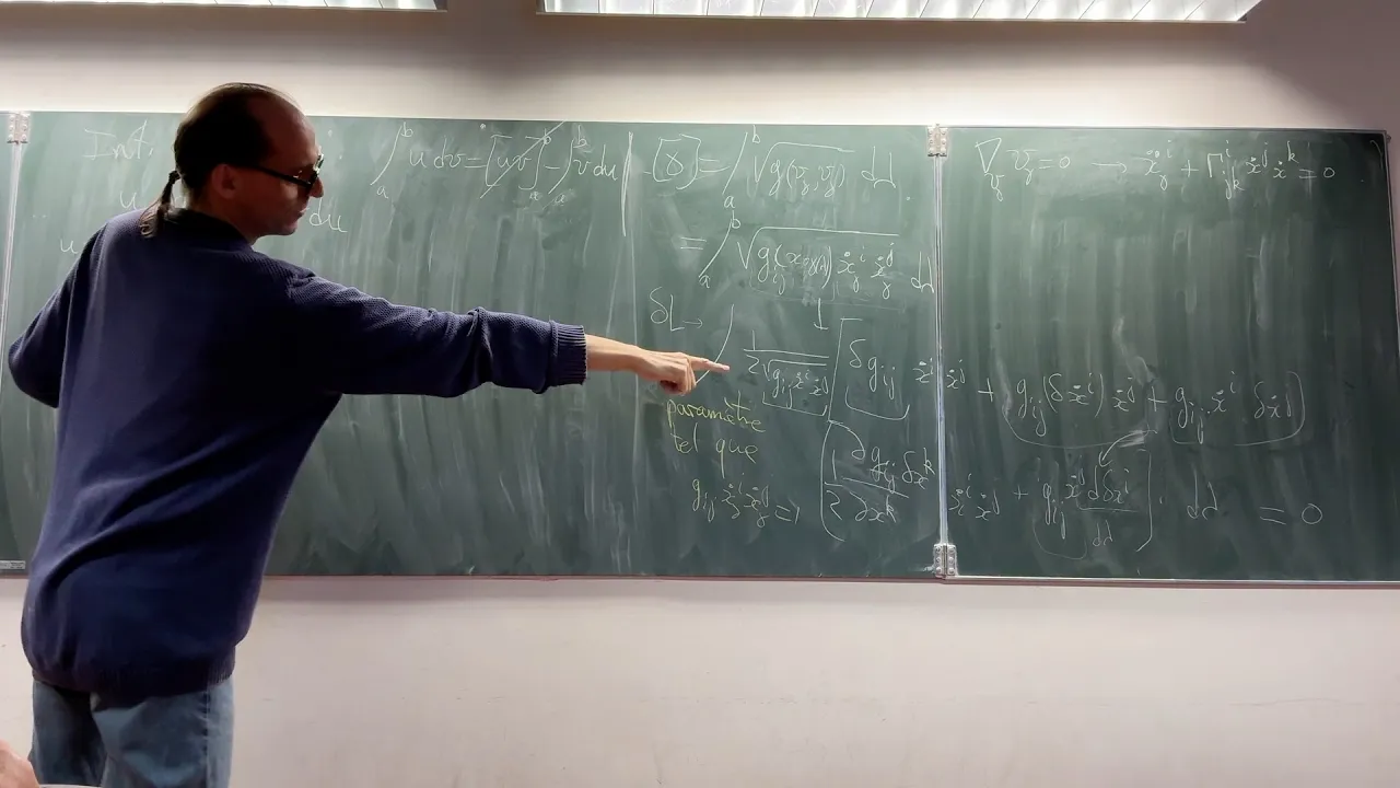

![[GR lecture 18/05/2022] 12: affine connection and covariant derivative](https://i.ytimg.com/vi/jPcrJ7RepLg/maxresdefault.jpg)
![[GR lecture 08/06/2022] 17, 18: geodesic deviation equation, SEP and electrodynamics](https://i.ytimg.com/vi/ot-GdF45IaE/hqdefault.jpg?sqp=-oaymwEmCOADEOgC8quKqQMa8AEB-AH-CYAC0AWKAgwIABABGGkgaShpMA8=&rs=AOn4CLC8gFu9rsvSsgTc-EGOz4zQgxMDzA)


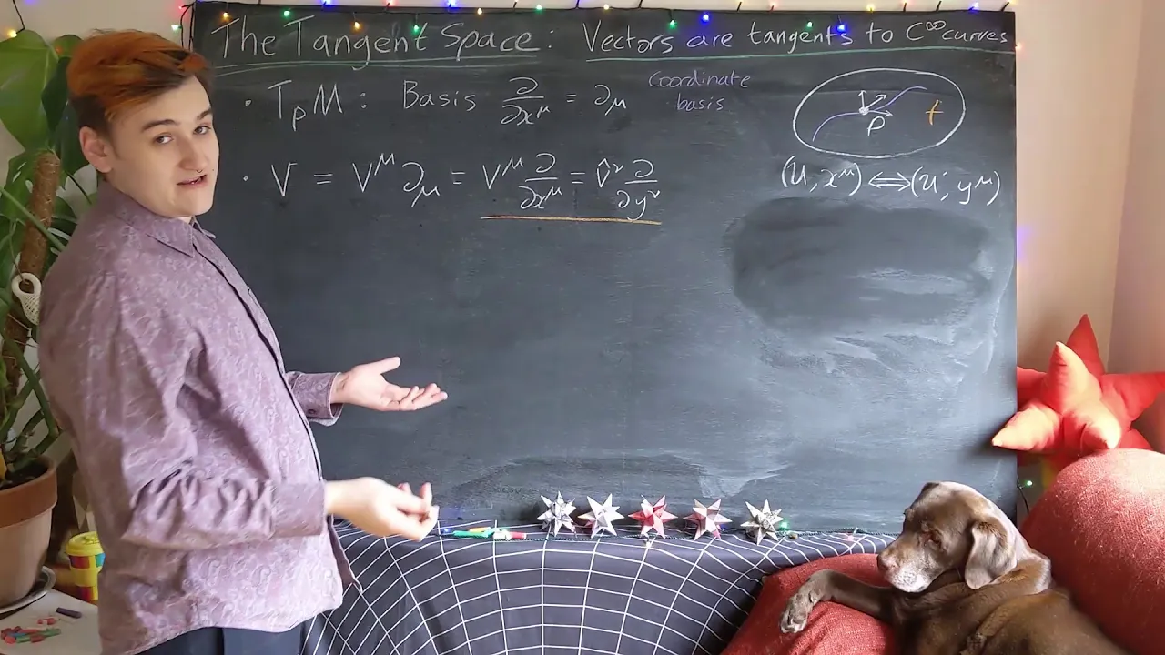

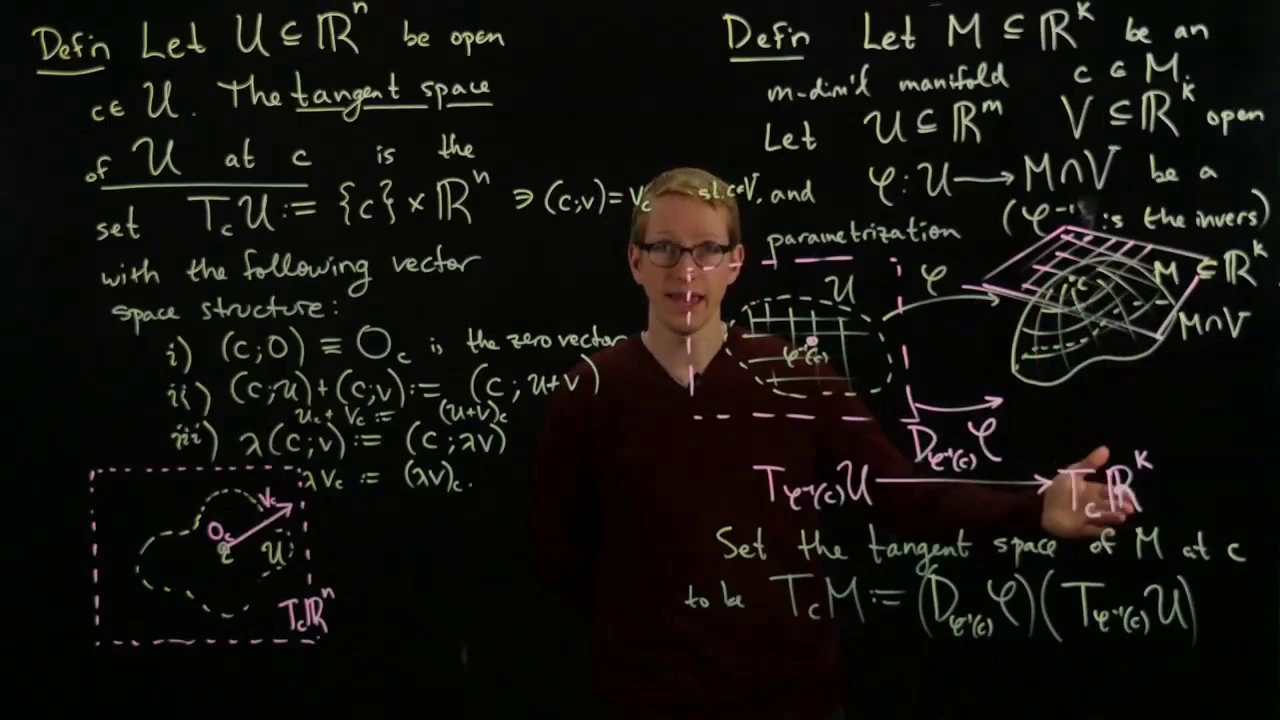
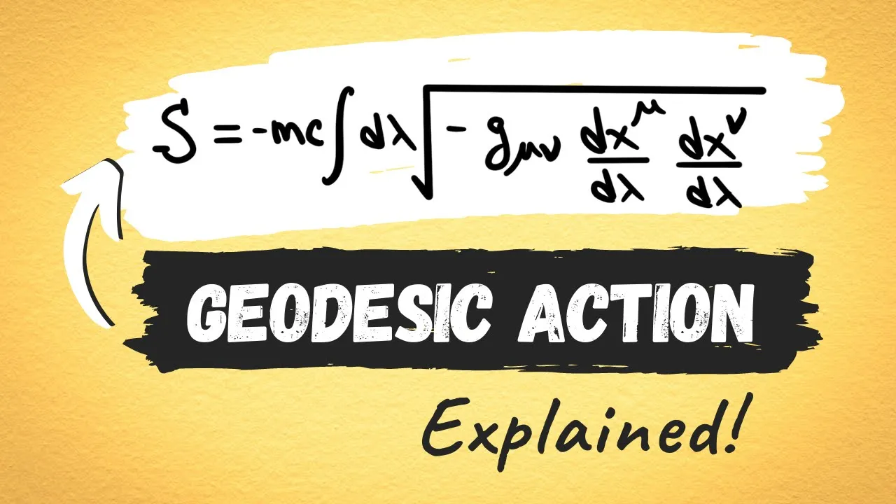


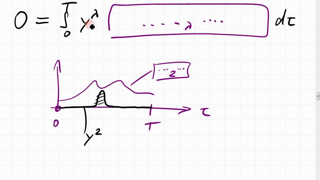
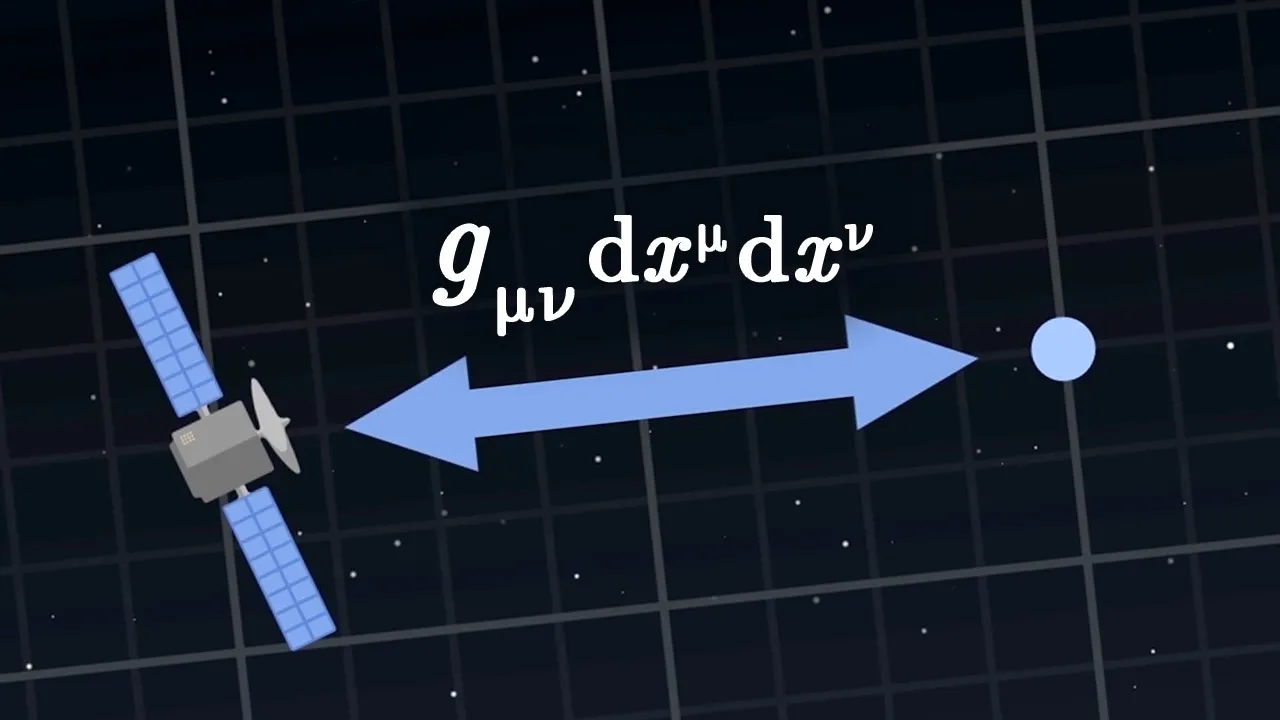
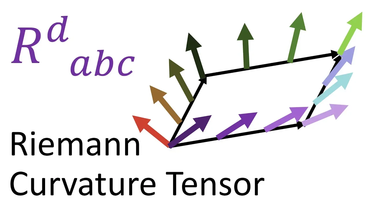


![[다변수 미적분 심화 스터디] Connection에서 Riemannian curvature tensor로](https://i.ytimg.com/vi/snNrsEnaURA/maxresdefault.jpg)



![12 - Curso de Relatividad General [ Transporte Paralelo (2/3) ]](https://i.ytimg.com/vi/vtGekOjTrZw/hqdefault.jpg)
Christoffel symbols are the unique connection coefficients that satisfy both torsion-free symmetry (Γ^ρ_μν = Γ^ρ_νμ) and metric compatibility (∇_α(g^μν) = 0), derived by applying the covariant derivative definition to the metric tensor and solving the resulting equations through index permutation and contraction with the inverse metric, yielding Γ^λ_μν = ½g^λα(∂_μg_να + ∂_νg_αμ - ∂_αg_μν).
Tensor Calculus for Physics: Christoffel Symbols Derivation
Added:Fundamental tensor algebra, including coordinate transformation laws and the distinction between covariant and contravariant indices.
The definition and role of the Metric Tensor, including how it defines inner products, distances, and is used for raising and lowering indices.
The concept of the Covariant Derivative as a tool to differentiate tensor fields on curved manifolds.
Basic differential geometry concepts, specifically differentiable manifolds, tangent spaces, and coordinate bases.
The Geodesic Equation, which uses Christoffel symbols to model the paths of particles in free fall through curved spacetime.
The Riemann Curvature Tensor, which measures geometric curvature by taking derivatives of the Christoffel symbols.
Einstein's Field Equations, showing how the metric tensor and connection coefficients relate to mass-energy density in General Relativity.
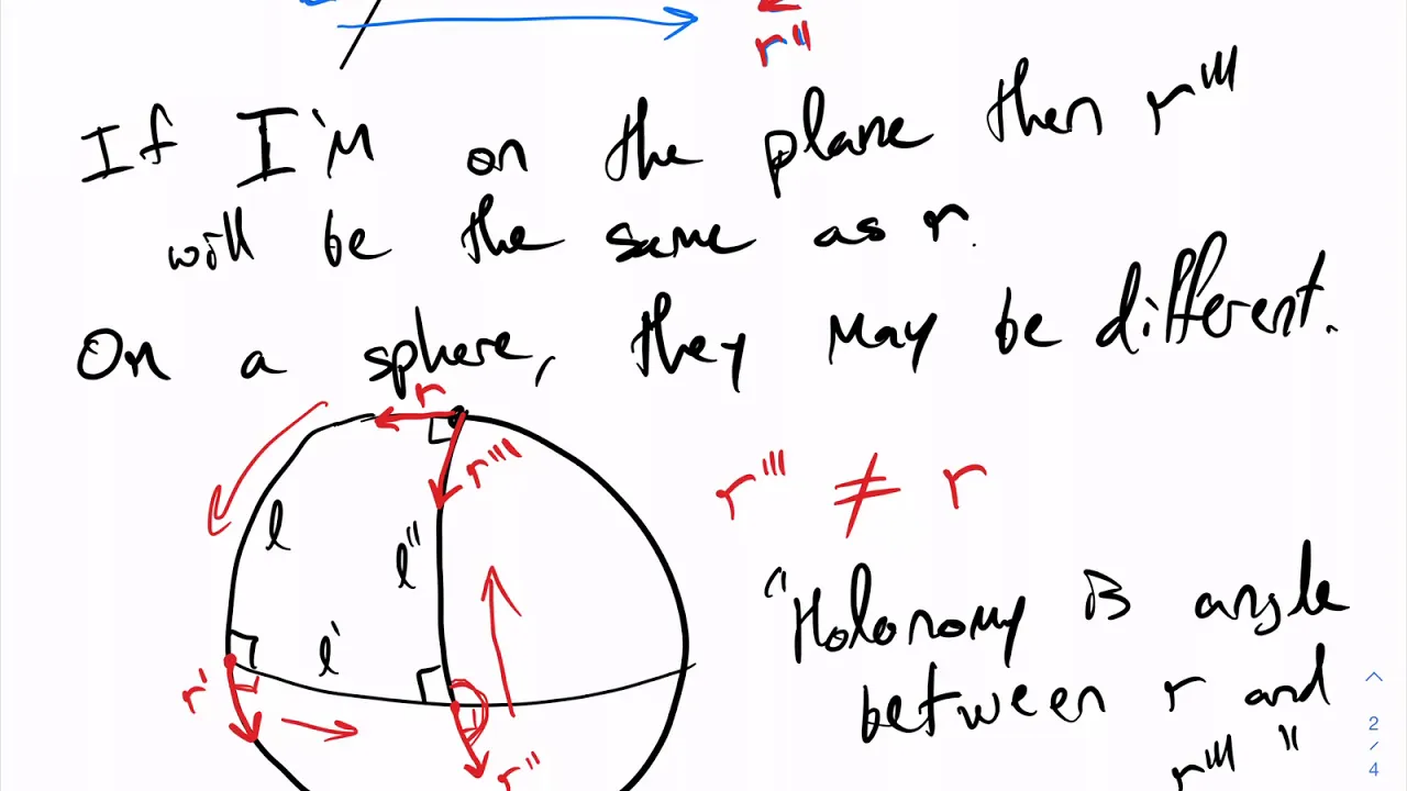
Parallel Transport and Holonomy, exploring how vectors behave when moved along closed loops in curved spaces.
50.8K views1.3Klikes17:05Original Release: 2020-03-16
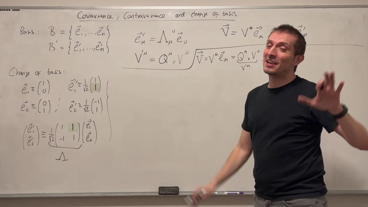
what's going on smart people it's been a while but it is finally tensor time again I'm in a different setting now in the last video which is probably like six months old at this point we defined the covariant derivative we noticed that if you take the derivative of a tensor the end result in general doesn't transform as a tensor anymore but if we add to it this additional linear transformation on the vector where these transformation coefficients are the affine connection coefficients the combination of the two does transform as a tensor so we modified our definition of the derivative to be the covariant derivative and in doing so now we're guaranteed that when we take covariant derivatives of tensors the end result will still be a tensor that's where we left off and as it stands this still isn't the most useful this is great we know that it transforms as a tensor that so tensor calculus saved but we still don't know what these coefficients are we just know how they transform but we self don't know what they are and one basis to be able to say what they are in a different you know you know I'm saying the only thing we've really imposed as of yet and if you look in Walt's book there's a bunch of little things that we've also been imposing implicitly along the way but all we've really been focusing on is the fact that there's no torsion we're imposing that there's no torsion which means that this set of connection coefficients is symmetric under the exchange of the bottom two indices if we swap alpha and beta these coefficients are the same that's the norm torsion rule and that narrows it down from infinitely many sets of connection coefficients to probably still infinitely many so the goal for today is to impose one more requirement that will narrow that down to one unique set of connection coefficients that we're going to call the Christoffel symbols okay and the requirement that we're going to impose I'm going to erase this because today we're not going to be taking covariant derivatives of vectors we're going to be taking covariant derivatives of second-rank tensors and the rule is a little bit different for that you see for every index that you take the covariant derivative or that the object you're taking the covariant derivative has you have one additional term of these connection coefficients and it carries a positive if the index is upstairs if it's contravariant and it carries a minus sign if it's downstairs so we're going to be taking the covariant derivative of a second-rank tensor enabling the metric tensor and to do that it goes as follows the covariant derivative we use alpha of some tensor is equal to that partial derivative still partial alpha since these are both downstairs it's going to carry a minus sign with the connection coefficients and we're going to be transforming each of the indices so that's why there's two terms so it's gonna do minus gamma I'm gonna just sum over the top index I'll call that row and we're gonna have an alpha that survives and then we're gonna interchange these mu and news for each term T Rho nu and then the next one we're just gonna swap this mu nu minus gamma Rho alpha nu T Rho mu great so this is how we take the covariant derivative of a second-rank doubly covariant tensor if these were upstairs then both of these would be positive if one was upstairs was downstairs wouldn't be positive one will be negative you get it the additional constraint that we're going to impose that allow us to uniquely solve for these connection coefficients is known as metric compatibility we write that up here metric compatibility and what that means is that the covariant derivative of the metric G mu nu should be equal to zero why should it be equal to zero all in some sense that's a choice but the way that I like to think about it is locally you think of the metric in terms of the dot products of the basis vectors so what we have is we have a derivative of a dot product is a derivative of a scalar product so it's just saying that when we parallel transport the basis vectors the dot product is left unchanged okay so this is something that we're gonna win pose and we're gonna do it three times we're gonna look at three permutations of this condition and they're all going to be equal to zero so we have what do we have Alpha Mu nu the hardest part of this whole thing is just keeping track of the indices but this is like episode 13 if the tensor calculus series so I assume that's that's always the hard part okay so for the first one we're gonna look at let's write it up here Alpha Mu nu we're gonna look at new new alpha and alpha so what we're gonna be doing is we're gonna be writing down the definition of the covariant derivative of the metric three times and then we're going to subtract those from each other since they're all equal to zero anyways so for the first one we're just we're always just going to be using this definition we're gonna swap our indices around for each term and we're going to switch this team you know to a team you knew so we have the partial derivative let's go ahead and already set this equal to zero so we have just so it's in our mind we have the partial derivative with respect to alpha of G mu nu easy part - now we need the connection coefficients we need to contract with the upper index since the metric is doubly covariant so when you sum over the top index so we'll row here the first index always survives in the connection coefficient so it's gonna have an alpha and then we're gonna have two terms one that has mu here one that has a new here you G summing over Rho nu minus gamma Rho alpha nu G Rho mu okay that's the first term let's do this two more times so if zero is equal to the partial with respect to MU this is where it gets tricky for me just because I've already written it down once so any other order just sounds like I'm doing it wrong in my head G nu alpha minus gamma to keep this row them you should always survive now and then we're gonna have a new G row this Gamma Rho you always survives alpha G real you getting better at this Rho nu survives so we'll have an alpha Rho mu minus Rho nu mu G Rho alpha there we go congratulations we've written the same thing three times now what we're gonna do I'm going to call this equation one this equation two and this equation three and we're going to take 1 minus 2 minus 3 this is the conventional way of coming up with these Christoffel symbols I don't know how they figured out to take these orders of indices the book does it a little bit different actually they define it twice in the book in different chapters but it all amounts to the same thing but this is how I learned it so this is how I'm teaching it so we take this difference of equations the derivatives will always survive so let's go ahead and just write those out real quick and I'm gonna partition this up a little bit just to make things a bit more a bit less cluttered and I suppose let's do it down here just because this is gonna be a bit lengthy I think so we have these partial derivatives I'm just gonna be rewriting those alpha G nu minus mu nu alpha minus nu nu and then we're going to be subtracting all of these connection coefficients terms but the reason we do this is because there's going to be a lot of cancellations so here we have a minus alpha mu here we have a minus mu alpha so if we take this minus this that this is symmetric about the bottom two indices so this is the same as minus alpha mu instead then these terms cancel when we take this minus this minus sign flips and we add it to it so this term cancels okay but not only that we have a minus let's see minus alpha nu and then we have a minus nu alpha same thing happens we have minus minus minus of these cancel as well okay so we have for cancellations out of the six terms that contain the connection coefficients okay and we're doing minus 2 minus 3 so this term gets multiplied by minus 1 so we have a neo nu plus because it's minus plus a nu mu but these can be permuted as well so this will just give us an extra factor of 2 times this okay so this is going to be a plus 2 Gamma Rho mu nu G Rho alpha so just the fact that I've swapped these indices this already gets multiplied by a minus 1 here and we get minus minus so it just becomes a 2 okay and this should be equal to 0 fantastic now we're gonna start solving for this gamma it's not going to be too hard all we're gonna have to do is recall our buddy old pal the inverse metric but let's go ahead and just get this stuff over on one side and the factor of 2 while we're at it so we have Gamma Rho mu nu G Rho alpha is equal to 1/2 and then we're moving this over so these two negatives become a positive so we get it D mu gene you alpha plus 2nu G alpha u minus this guy but we want to get this by itself so we're gonna impose a relation that we learned about when we defined the inverse metric which is that so where we have Rho alpha we're summing over Rho so in order to get a Kronecker Delta out of this I'm gonna have to contracted with an inverse metric that has an alpha in there so we can use G lambda alpha G Rho alpha is equal to I'm gonna get myself a little bit of space is equal to Delta Lambda ROH okay so these these are matrix elements these are these are numbers so the numbers commute with the connection coefficients which is 1 when I multiply by the inverse metric I can move it past this connection coefficient plus it's not being contracted with this guy yet well yeah no it's not because it doesn't carry any mutual indices so when we multiply this by the connection coefficient Rho mu nu all this does room new is it changes this row to Atlanta ok so multiplying both sides by the inverse metric we get our expression for the connection coefficients gamma lambda mu nu is equal to one-half G lambda alpha D mu G nu alpha D nu G alpha u minus D alpha G yeah yeah there we have what are defined as the Christoffel symbols I'm not going to try to spell Christoffel or symbols no this is called the Christoffel symbols of the second kind if we lower the lambda index then it's called the Christoffel symbols of the first kind for some reason I don't quite understand that but it is what it is so now we've uniquely defined the connection coefficients in terms of the metric so one thing and in a sense we're done this video is done in the next video what we're going to be talking about is more complex differential operations acting on tensors namely divergence curl laplacian x' now that we know how to actually calculate these coefficients if we know what the metric is just a couple more comments before we wrap it up when people learn about Christoffel symbols oftentimes the first thing that you start associating Christoffel symbols with are curvatures of space because you have this derivatives of metrics and stuff like that but that's not really the right way to be thinking about this we will in a couple videos develop a formalism for determining whether or not the space that we're working in is curved or not what we talked about the Riemann curvature tensor but nonzero Christoffel symbols does not necessarily mean that your space is curved now if we're working in a just to forget about x they're just a Cartesian basis in you know flat space then we know that our metric where'd my chalk go we know that our metric Genia new is just a diagonal once right in Cartesian coordinates and flat space this is our metric so when we take derivatives of the metric we get zero every single time so you might say oh flat space the Christoffel symbols are 0 but if we are in safe spherical coordinates where we have an r-squared here now and are squared sine sine theta I always forget if it's squared or not now we're taking derivatives with respect to R with respect to theta of this guy here so the Christoffel symbols actually won't be 0 even though the geometry of the space hasn't changed at all only the basis that we're describing it in has and the reason for this and this is an appropriate way of interpreting the Christoffel symbols in flat space but you have to be more careful when we actually do start dealing with curvature is when we take derivatives of vectors we have coefficients attached to basis vectors right those coefficients might change depending on where we're looking at in space but also the basis vectors might change and that's what's characterized by these connection coefficients if I have say something on the surface of a circle and I have my polar coordinates where I have my basis vector here my R hat and I have my theta hat or let's just make them not normalized in gr you typically don't have the normalized basis vectors these basis vectors change depending on where along the circle on path so in a Cartesian coordinate system when I take these derivatives or what I measured these points at different are these vectors at different points the basis vectors themselves don't start pointing in different directions but in polar coordinates they do so that's what's being captured in in a flat space by these Christoffel symbols that's also why when you look in Griffiths or when you start dealing with divergence curl laplacian x' and these different coordinate systems you can't just take derivatives with respect to the coordinates you have these additional factors and these additional factors are actually contained in these Christoffel symbols but while beginning to that in the next video next video we'll talk about divergence curl and laplacian or the covariate generalizations of those in terms of covariant derivatives and then in the following video we are I haven't thought about it yet but I imagine we'll start commuting covariant derivatives will define the Riemann curvature tensor I hope but I hope you guys enjoyed this video learn something let me know in the comments section if you did and I'll see you guys there
Up Next

14:20
Geodesic Equation Derivation | Tensor Calculus & General Relativity
@FacultyofKhan
12K views•2024-10-26

12:53
21cm Hyperfine Transition in Neutral Hydrogen: Radio Astronomy Basics
@AaronRobertParsons
12.4K views•2011-10-13

35:23
Deriving the Einstein Field Equations | Tensor Calculus Finale
@AndrewDotsonvideos
29.6K views•2021-04-15

27:14
Entropy and the Second Law of Thermodynamics Explained
@veritasium
27.5M views•2023-07-01
Related Study Plans & Knowledge Roadmaps
Structured learning paths in Physics
physics
Nuclear Physics (Decay, Fission & Reactors)
01Atomic Structure and the Binding Force
02Radioactive Decay and Half-Life
03Nuclear Fission Mechanics and Chain Reactions
+ 2 more learning modules
12h5 modules
Explore Roadmap
physics
Soft Matter (Polymers, Colloids & Rheology)
01Foundations of Soft Matter & Thermal Forces
02Polymer Physics and Macromolecules
03Colloids, Surfactants, and Self-Assembly
+ 2 more learning modules
38h5 modules
Explore Roadmap
physics
Analytical Mechanics: Lagrangian & Hamiltonian
01Mathematical Foundations: Calculus of Variations
02From Newtonian Mechanics to Constraint Dynamics
03The Principle of Least Action & Lagrangian Mechanics
+ 3 more learning modules
28h6 modules
Explore Roadmap
physics
General Relativity (Spacetime & Cosmology)
01Foundations of Relativity: Special Relativity
02The Geometry of Spacetime: Equivalence Principle & Curvature
03Einstein's Field Equations: The Mathematics of Gravity
+ 2 more learning modules
55h5 modules
Explore Roadmap