















![ДИВНА МАТЕМАТИКА ЕЙНШТЕЙНА 🤯 [VERITASIUM]](https://i.ytimg.com/vi_webp/QZQptiZOQfs/maxresdefault.webp)

The geodesic equation, which describes the shortest path between two points on a Riemannian manifold, is derived by minimizing the arc length functional L = ∫√(g_ij dx^i/dt dx^j/dt) dt using the calculus of variations and Euler-Lagrange equations; this yields the second-order differential equation d²x^p/ds² + Γ^p_jk(dx^j/ds)(dx^k/ds) = 0, where Γ^p_jk are the Christoffel symbols of the second kind constructed from the metric tensor g_ij, and when parameterized by arc length s, the equation simplifies to the familiar form where the right-hand side equals zero.
Geodesic Equation Derivation | Tensor Calculus & General Relativity
Added:Calculus of Variations: Familiarity with functionals, extremizing path integrals, and deriving the Euler-Lagrange equations.
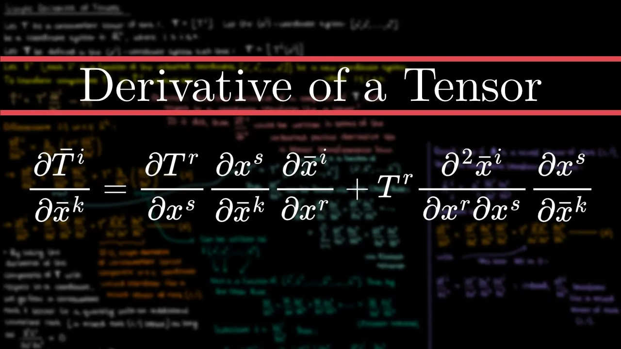
Tensor Algebra and Calculus: Understanding the metric tensor, coordinate transformations, and index notation (Einstein summation convention).
Differential Geometry Basics: Concepts of differentiable manifolds, tangent spaces, and the definition of curves on curved spaces.
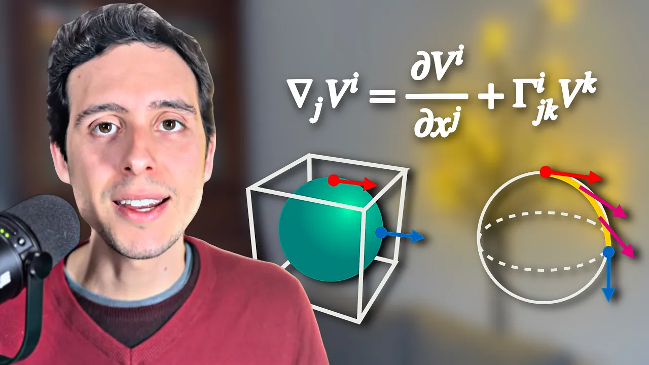
Covariant Differentiation: Understanding how to take derivatives in curved spacetime and the introduction of Christoffel symbols (connection coefficients).
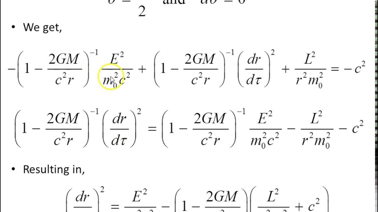
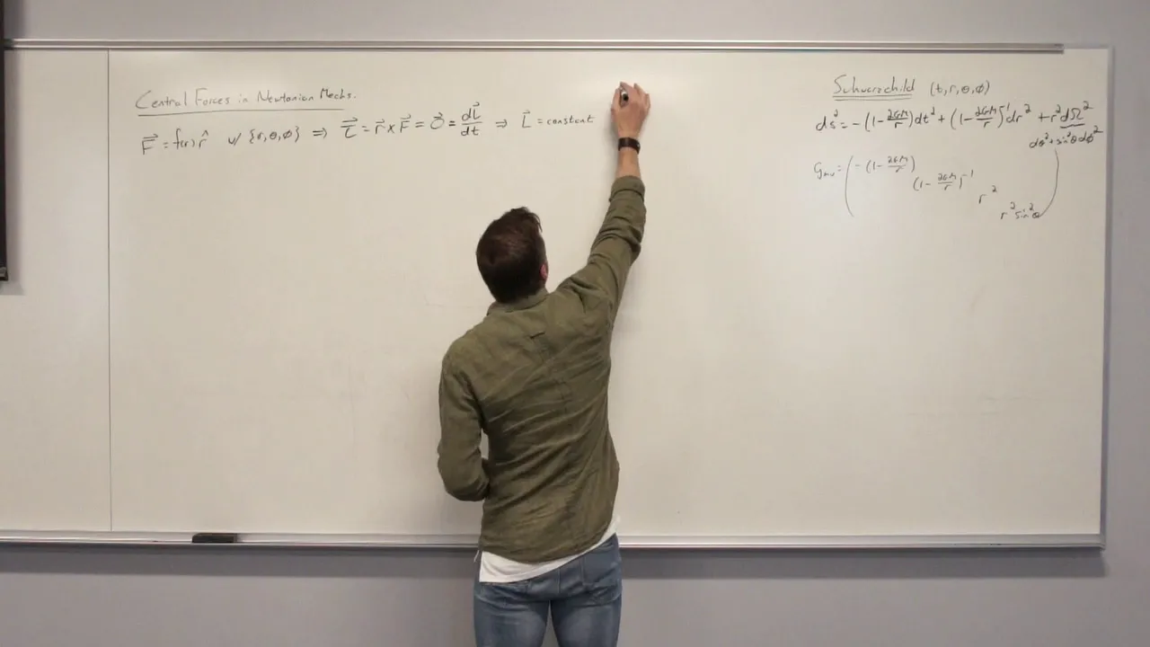
The Schwarzschild Geodesics: Applying the geodesic equation to calculate planetary orbits (such as the perihelion precession of Mercury) and the gravitational deflection of light.
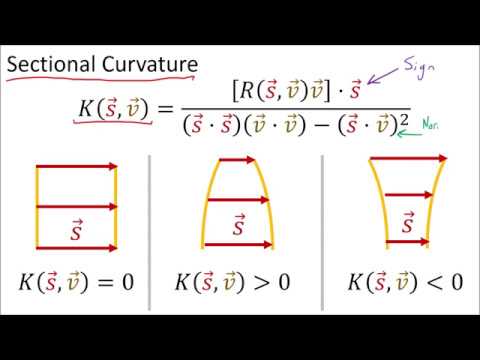
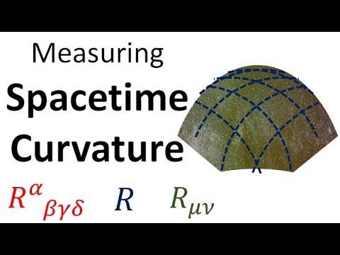
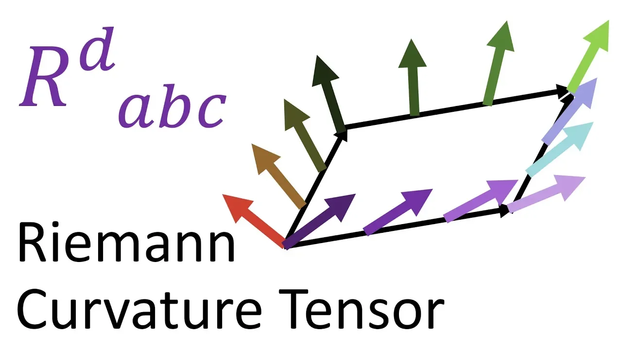
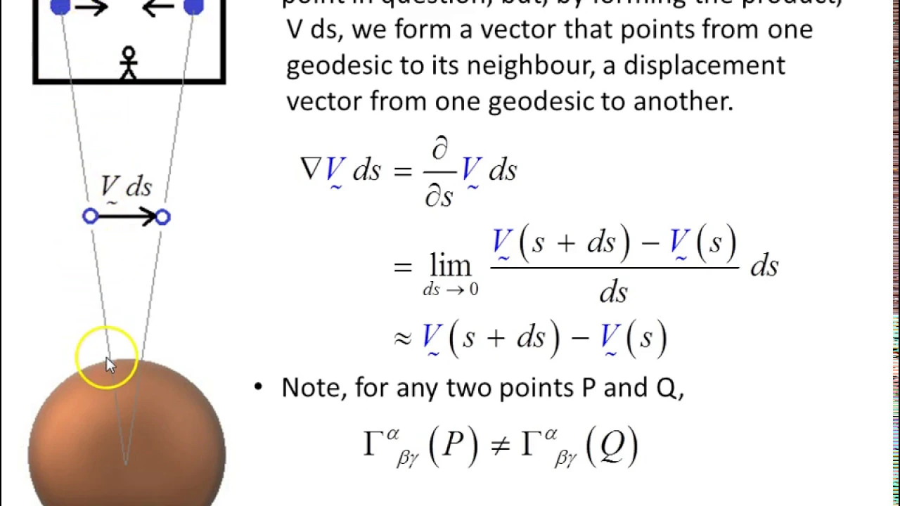
Geodesic Deviation: Exploring how neighboring geodesic paths diverge or converge, which defines tidal forces and introduces the Riemann Curvature Tensor.
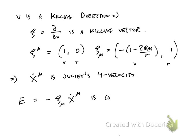
Killing Vectors and Conserved Quantities: Utilizing spacetime symmetries to identify constants of motion (like energy and angular momentum) along a geodesic.
Einstein Field Equations: Transitioning from how particles move in curved spacetime (geodesics) to how matter and energy curve spacetime itself.
12K views372likes14:20Original Release: 2024-10-26
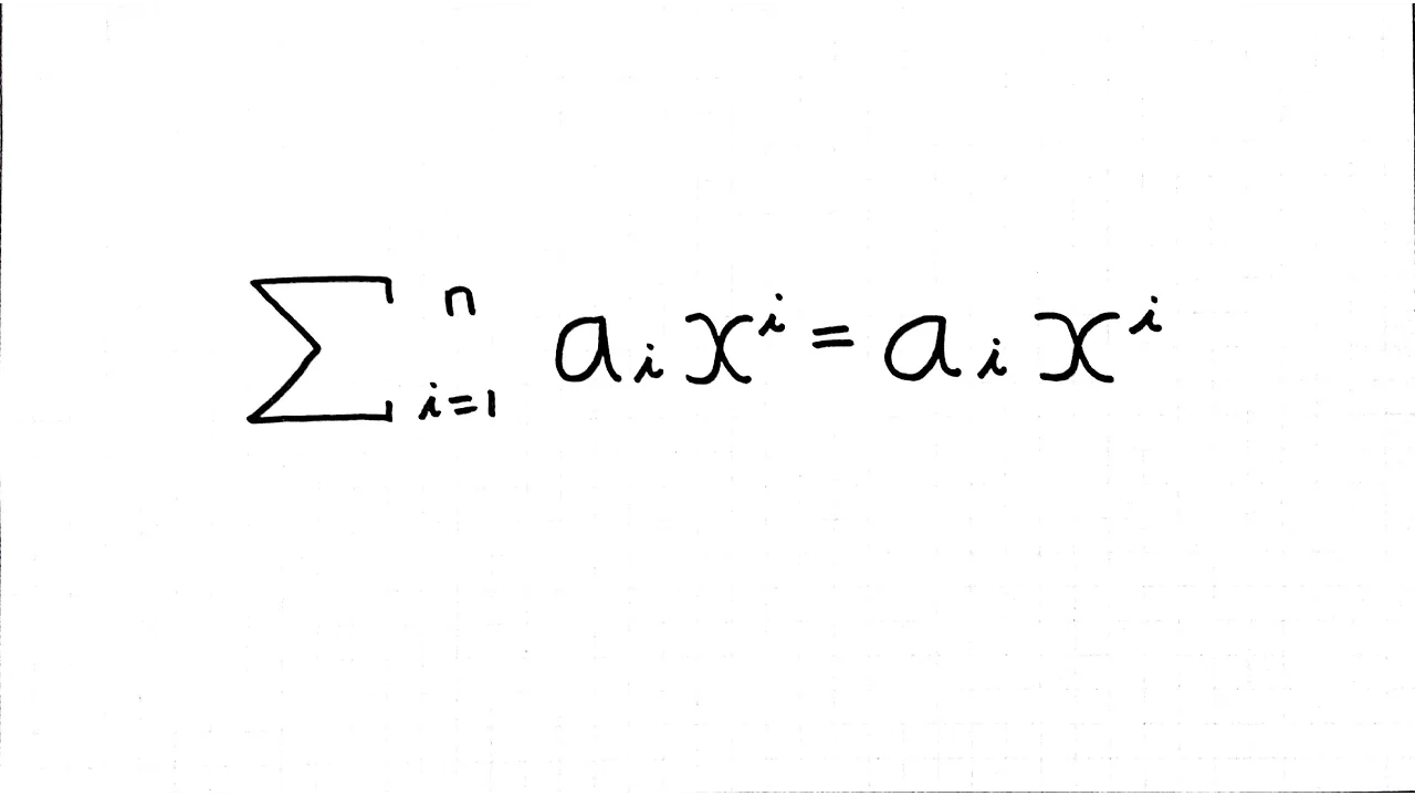
we finally made it boys and girls for the four women who actually watch my videos this far into my series on tensor calculus I'm going to derive probably one of the most important equations not just in tensor calculus but in differential geometry and probably what most of you are interested in general relativity we're going to derive the geodesic equation from first principles using what we've learned so far in tensor calculus suppose I have a curve gamma that's parameterized with respect to the parameter T in general this gamma can be written as a function of each of the coordinates so X Super One X super 2 all the way to x super n where n is the dimension of my space and since gamma is parameterized by the parameter T each of these coordinates that gamma is a function of is also a function of the parameter T suppose also that my curve gamma exists in a space and coordinate system with the metric tensor G whose components are given by G sub i j if I wanted to find the length of gamma from tal a to tal B then I can find this length which I'll call L using this integral the integral from A to B of the square root of the absolute value of G sub i j times the derivative of x super I with respect to ttimes the derivative of x super J with respect to T where x super I and x super J are the parametric equations of some coordinates that are found in the curve gamma later on in the video you'll see that this absolute value will disappear and that's because I'm going to assume the metric tensor is positive definite meaning that the term inside the absolute value will not be negative so we can later just get rid of the absolute value the positive definite nature of the metric tensor is generally true for most situations that we'll be dealing with specifically situations in ronian Geometry anyway let's analyze this term inside the integral a bit and pull it out to the side both the indices I and J are repeated twice in this expression so according to the rules of Einstein notation this means that these indices are summed over because these indices are summed over they're summed out so what I'm left with is a scalar quantity which I'll call W which doesn't have an index because the indices I and J are just summed over now let's take this length integral and approach things slightly differently instead of trying to find the length of the curve I want to find the curve that minimizes this length integral that is I want to find the parametric equations for the coordinates all the X Super One X super2 and so on that minimize this length functional L this function of functions the curve that minimizes the length functional between two points is called a geodesic curve for that particular space you'll also hear people pronounce it as geodesic now how do I minimize my length functional how do I minimize a function of functions or at least find a function which makes a functional stationary well I use the techniques of calculus of variation specifically I need to use the oiler lrange equation let's now go back and recall some Concepts from variational calculus recall that if I have an integral I of a function X Y and Y Prime prime or Dy by DX if I want to find a function y ofx which minimizes this I which effectively is a function of functions then the way to find the stationary function y is to solve for it using the oiler lrange equation which would look something like this in this case but if I had a more complicated functional which involved an integral of a function of T and multiple dependent variables and their derivatives then to make this functional stationary I would still have to solve the oiler lrange equation but I would need to solve it for each dependent variable so X Super One X super 2 all the way to x super n now this generic length integral with the metric tensor and everything this term being integrated in the generic length integral is also a function of T in multiple dependent variables our parameterized coordinates x super one and so on and the derivatives of these parameterized coordinates with respect to T So if I want to minimize this length integral I need to apply the oiler lrange equation to each of these parameterized coordinates so in general if I write the function I'm integrating in this length integral as capital F of t x super1 the T derivative of x super one all the way to X supern and its derivative then if I want to find the coordinate X Super K that minimizes this length functional I would have to solve this Oiler lrange equation for x Super K where K is some free index that can be anything from 1 to n depending on the specific parameterized coordinate you're interested in I'm going to call this equation one now this Oiler Lage equation is just the generic equation for finding the X Super K coordinate if I wanted to find the complete curve gamma I'd have to solve the equation one for every value of K so from 1 all the way to n so if I wanted to find my complete length minimizing curve gamma I'd need to solve a system of n different Oiler lrange equations for each parameterized coordinate so hopefully that makes sense let's now plug in some values this function capital F can just be written as the square root of w which I defined up here that means if I wanted the partial of capital F with respect to X Super K I can use the chain rule to show that in terms of w this partial derivative is just the following I can do the same thing for the partial of capital F with respect to X Super K prime or DX Super K by DT and this is what it would look like in terms of w if I apply the change Rule now let's bring back our W this W consists of G sub i j and the T derivatives of x super I and x super J among these terms the T derivatives of x super I and x super J are just functions of T the coordinates and their Ives obviously can't be functions of each other however the metric tensor component G sub i j is in general a function of the coordinates one of which will be X Super K this means that when I'm taking the partial of w with respect to X Super K these T derivatives are effectively constants for that partial derivative and all we would have is the partial of G sub J times these two t derivatives in the first term of this Oiler lrange equation but what about the second term particularly the partial of w with respect to X Super K Prime well this is a bit more tricky we'll bring in our W again which is a product of G sub i j and the T derivatives of x super I and x super J now G sub i j is only a function of the coordinates it is not a function of the T derivatives of those coordinates so you might be tempted to say here that since there's no derivative of x Super K the partial of w with respect to X Super K Prime is zero but that's actually not true that's because this W is actually a summation of this term on on the right which is a sum over both the I and J indices some of the terms that show up in the summation actually include x Super K Prime particularly G sub i k times the T derivative of x super I and X Super K and G subki itimes the T derivative of x Super K and x super I so since these two terms actually contain X Super K Prime the partial of w with respect to X Super K Prime would be the sum of these two terms and finally since the metric tensor is a symmetric tensor the G sub Ki component equals the G sub i k component so we can actually combine these terms to get twice the value of a single term so now if we plug this into our Oiler lrange equation for our GOC curve this is what we get note that I've moved the derivative and T term to the other side of the equality here and speaking of this derivative and T term let's evaluate it we'll need to use the product rule on the W term the G sub i k term and the T derivative in the x super I term when we do that this is what we get let's leave the DW by DT term as it is for now and focus on the T derivative of G sub i k in general we know that the metric tensor component is just a function of the coordinates X Super One X super2 and so on each of these coordinates we know is a function of T So if I want the total derivative of G sub i k with respect to T then by the chain rule it would just be the partial of G sub i k with respect to X Super 1 time the derivative of x Super 1 with respect to t plus the partial of G i k with respect to x super 2 time the derivative of x super 2 with respect to T and so on and so forth I can simplify this by Einstein notation by using J as my dummy index to express this long expression as the sum over J of the partial of G sub i k with respect to x super J time the T derivative of x super J when I perform the simplification this is what I get with my Oiler lrange equation now I'm going to do three small things I'm going to multiply both sides by the square root of w so effectively canceling that out and I'm going to multiply both sides by two and then move the W containing term to the left and everything else without the W to the right when I do that this is what I end up with now what we'll do is split up this 2 * G sub i k term on the right since G sub i k is the same as G sub Ki by the symmetric nature of the metric tensor I can rewrite the second term in my split as G subki now I'm going to pull off another trick in this first term with the G sub I the indices I and J are dummy indices because they're repeated twice and since they're dummy indices I can replace them with almost any index I want except maybe K and it wouldn't change my expression because I and J just get summed over they're dummy indices so what I'll do is that I'll replace the I by the J and the J by the I because that'll make things more simple for us later on when I do that my Oiler lrange equation ends up like this now all three of these terms with the derivative of the metric tensor component are also all multiplying the derivatives of x super I and x super so if I take these x super I and x super J derivatives common here's what I'll have now does this term involving the derivatives of the metric tensor components look familiar well it should because by definition this is just two times the christopal symbol of the first kind with indices JK when I plug this christopal symbol in this is what I'll get let's now simplify this equation further by multiplying both sides by the components G super PK of the inverse metric tensor and we'll also flip our equation from left to write for convenience when I do that this is what I end up with the nice thing about this equation is that I can simplify things even further the product of the metric tensor component G sub I with the inverse metric tensor component G super PK is The Chronic or Delta symbol with the indices pni meanwhile the product of G super PK and the christopal symbol of the first kind with indices ik JK is just the christopal symbol of the second kind gamma super p and then sub J and this is just from from my video on christopal symbol so go watch that if you haven't already now the chroner Delta symbol is zero except when I equals P where it's just one so when I replace the i in these terms by P and when I divide both sides by two I get the equation that I've been looking for this whole time this geodesic equation let's analyze this equation a bit what this tells me is that if I plug in a metric tensor which basically goes into my christopal symbol and into my w term on the right then I can find the geod between two points corresponding to that metric tensor and the geodesic I would solve for with this geodesic equation would be a curve parameterized with respect to the parameter T So if I plug in say the metric tensor for ukian space and cartisian coordinates I would be able to find the parametric equations for the corresponding geodisc which in this case is just a straight line the shortest distance between two points in standard ukian space is a straight line similarly if I plug in the metric tensor for the surface of a sphere into the geodesic equation I would be able to find the parametric equations for that geodic which would just be an arc on the great circle in general I can do this for pretty much any metric tensor corresponding to any space or coordinate system and I can get my corresponding geodesic now what if I told you that I can simplify things even further the way it's structured right now my geodisc equation which I'll call equation two would give me the equation of a curve that's parameterized with respect to T but if you recall my differential geometry videos we often like to have our curves parameterized with respect to AR length because that makes our algebra simpler so what if I wanted the solutions to my geodic equation to be parameterized with respect to Arc Length well in that case the geodic equation simplifies even more let's bring back our length integral you can also write this length integral as the integral from point A to point B of the arcl length element DS in that case this square root term would just be written as DS by DT because I have the DT outside which would mean that my w is just the square DS by DT now if my curve were already parameterized with respect to Arc Length then that would mean that the parameter T is just the Arc Length s and if W is the derivative of s with respect to the parameter t^2 then W would just become the derivative of s with respect to S which is just one and since W is now a constant when we have the parameter become the Arc Length s it's derivative with respect to a parameter s in this case would just be zero so in equation two parameterizing with respect to arc length makes your right hand side zero this greatly simplifies the geodic equation to the second derivative of x super p with respect to S Plus the christopal symbol of the second kind gamma super P sub J times the derivative of x super I with respect to stimes the derivative of x super J with respect to S equals z this is often quoted as the geodesic equation that most are familiar with but it's not a single equation it's a system of differential equations that for a given given metric tensor which is incorporated into the second kind christopal symbol will spit out a parametric equation describing each coordinate in the geodesic curve the curve that minimizes the distance between two points this time though the parametric equation will be written in terms of the arc length parameter s now one caveat to all this is that the oiler lrange equations gives you a function that makes a functional stationary you don't necessarily know that that function makes that functional a minimum just by solving the oiler lrange equation but this is something that you've probably come across if you've seen my calculus of variations video I'm very careful to specify that distinction so there you have it I've officially derived the geodic equation I'd like to thank the following patrons for their support and if you enjoyed the video feel free to like And subscribe this is the faculty of KH signing out
Up Next

36:21
General Relativity: Manifolds, Covariant Derivative, and Geodesics
@eigenchris
115.7K views•2021-05-11

12:53
21cm Hyperfine Transition in Neutral Hydrogen: Radio Astronomy Basics
@AaronRobertParsons
12.4K views•2011-10-13
6:58
Minkowski Diagrams Explained: Special Relativity Basics
@FacultyofKhan
6K views•2023-11-06

27:14
Entropy and the Second Law of Thermodynamics Explained
@veritasium
27.5M views•2023-07-01
Related Study Plans & Knowledge Roadmaps
Structured learning paths in Physics
physics
Nuclear Physics (Decay, Fission & Reactors)
01Atomic Structure and the Binding Force
02Radioactive Decay and Half-Life
03Nuclear Fission Mechanics and Chain Reactions
+ 2 more learning modules
12h5 modules
Explore Roadmap
physics
Soft Matter (Polymers, Colloids & Rheology)
01Foundations of Soft Matter & Thermal Forces
02Polymer Physics and Macromolecules
03Colloids, Surfactants, and Self-Assembly
+ 2 more learning modules
38h5 modules
Explore Roadmap
physics
Analytical Mechanics: Lagrangian & Hamiltonian
01Mathematical Foundations: Calculus of Variations
02From Newtonian Mechanics to Constraint Dynamics
03The Principle of Least Action & Lagrangian Mechanics
+ 3 more learning modules
28h6 modules
Explore Roadmap
physics
General Relativity (Spacetime & Cosmology)
01Foundations of Relativity: Special Relativity
02The Geometry of Spacetime: Equivalence Principle & Curvature
03Einstein's Field Equations: The Mathematics of Gravity
+ 2 more learning modules
55h5 modules
Explore Roadmap