General Relativity: Manifolds, Covariant Derivative, and Geodesics

[00:00:00]in this video we're going to see how the equivalence principle leads to space-time being a manifold which is just a fancy way of saying that space-time is curved i'm going to warn you right now that this video is more like a brief survey of the topics of manifolds covariant derivatives and geodesics i'm covering a lot of complicated topics in a very shallow way in a really small amount of time by the time you're done watching this video i only expect you to have a very basic idea of what all these terms mean but i don't expect you to really fully understand them if you feel like you need more time with these topics i have several hours worth of videos in my tensor calculus series linked in the description that you can check for more information you're free to skip ahead to the next general relativity video if you want but if you're finding the mathematics really confusing as the videos go on i would strongly recommend you come back and watch these videos on covariant derivatives and geodesics so that you can get a better understanding of them also in this video i will be using the einstein summation notation so when we have a summation over a summation index like mu we're going to leave the summation symbol out any time that we see a summation index repeated up top and down below we take this to mean that a summation is happening and we pretend that there's actually a summation symbol out in front so we know that the equivalence principle tells us two things number one in small regions of space-time falling inside of a freely falling box feels exactly like floating in deep space and number two in small regions of space-time sitting on a gravitational mass feels exactly like being in a rocket that's accelerating in a non-inertial frame the equivalence principle is basically telling us that in small regions of space time we can never detect the existence of gravity locally we could always attribute the effects of gravity to us being in an inertial or non-inertial frame in deep space far away from any masses we can only detect the existence of gravity in large regions of space-time where tidal forces come into play remember tidal forces appear when the pull of gravity is non-uniform objects at the same height that are falling towards a planet will get pulled together and objects that are falling at different heights will get pulled apart so because gravity can only be detected in large regions of space-time our new theory of gravity general relativity only applies in large regions of space-time in small local regions of space-time general relativity disappears and we're left with only special relativity so in small regions of space-time general relativity looks exactly like special relativity in other words general relativity is locally indistinguishable from special relativity as a result the curved space time of general relativity is locally indistinguishable from the flat space time of special relativity this brings us to the idea of a manifold a manifold is basically a curved space that looks flat in a small local region the most familiar example of a manifold is the surface of the earth at a large scale the earth's surface is basically a sphere which is curved but to us tiny people living on the surface the earth appears basically flat in a small local region in addition to spheres other examples of manifolds include cylinders and saddle surfaces these are all two-dimensional manifolds since they look like a flat 2d plane if we zoom in up close when a manifold has the concept of distance between two points we call it a riemannian manifold we measure distances using a special function g called a metric which takes two vectors and outputs their dot product in previous videos you've already seen that g acting on basis vectors gives the components gij of the metric tensor if we input the same vector twice into the metric the output is that vector dotted with itself which gives the squared length of the vector normally we expect the squared length of a vector to always be positive however if you watched the relativity 104 part e video you'd know that in space time time-like vectors have a positive squared length light-like vectors have a zero-squared length and space like vectors have a negative squared length when a metric can measure vectors to have positive zero or negative squared lengths we instead call it a pseudometric and a manifold with a pseudo-metric for measuring distances between points is called a pseudo-romanian manifold so in general relativity space-time is a manifold because it's a curved space that is locally flat because of the equivalence principle it's a four dimensional manifold because it has one time dimension and three spatial dimensions it's also a pseudo-romanian manifold because the space time metric that measures separation between points can give us squared lengths that are positive zero or negative positive squared lengths help us measure proper time between two points negative squared lengths help us measure proper distances between two points and zero squared lengths give us the paths of light beams now there are two different ways of thinking about manifolds these are the extrinsic view and the intrinsic view the extrinsic view means to look at a manifold from the outside when we look at the earth from outer space or look at these other surfaces like this we are looking at the manifold from an extrinsic point of view the extrinsic view is useful because it lets us use the surrounding space to describe the manifold for example if a car is on the earth we can invent a coordinate system with the origin at the earth's center and draw a position vector for the car also if the car is moving across the earth's surface along this path we can draw a velocity vector for the car which is tangent to the path it travels along notice that the origin the position vector and the velocity vector don't live directly on the earth's surface they instead live in the outside 3d space surrounding the surface but that's totally fine because we're working with the extrinsic view of the manifold which incorporates the surrounding space now what if we were not allowed to use the outside 3d space and we were forced to look at the surface of a manifold like this using a map this is called the intrinsic view of manifolds because we're forced to stay inside the surface and never talk about the outside space it's often harder for us to use intuition with intrinsic geometry for example using our eyes this map makes it look like greenland is much larger than australia but if we compare their actual sizes australia is actually much bigger with intrinsic geometry we can't measure size using our eyes instead we need to calculate distances using a formula that involves the metric the metric is the only thing we can rely on to have an accurate description of distances with extrinsic geometry the plane sphere cylinder and saddle are all clearly different but with intrinsic geometry all of these manifolds just kind of look like this they're just coordinate systems that all kind of look the same at first glance and these curves drawn on the manifolds all kind of look the same in the intrinsic view but in the extrinsic view we can see these curves are different because they live on different surfaces the shapes of these different spaces causes the curves to have different lengths this is because each manifold has a different metric that's used to calculate the lengths of the curves to get the length of a curve on a manifold we just integrate the lengths of the tangent vectors along that curve as we did in relativity 105 part d now when it comes to the general relativity that einstein introduced in 1915 the four-dimensional space-time manifold that is our universe is viewed intrinsically four-dimensional space-time exists on its own and it is not embedded in some higher dimensional space that's five-dimensional or six-dimensional when we draw a world line on a space-time diagram coordinate system for our four-dimensional manifold we cannot use our eyes to determine how long that world line is or whether or not the world line is straight instead we have to use the four-dimensional space-time metric to determine these things and the metric is given to us by the einstein field equations which we'll talk about in a later video so the only way to measure proper times proper lengths and determine the paths of light beams in space time is to use the metric so with the extrinsic view of manifolds we were allowed to use an origin position vectors and tangent vectors that all lived outside the manifold surface but for the intrinsic view of manifolds the outside space doesn't exist now it's possible to put the origin of our coordinate system as a point on the manifold but the idea of a position vector that connects the origin point to another point doesn't make sense anymore and we're going to have to get rid of position vectors when we study manifolds intrinsically on curved manifolds like the surface of the earth two points can be connected by a curve but they cannot be connected by a straight arrow since this straight arrow would leave the manifold and tunnel through the earth the same is true for the intrinsic manifold of space-time the four-position vector s that we've been using in flat space-time to identify events doesn't exist in the curved space-time of general relativity now what about tangent vectors in the extrinsic case if we had a curve parameterized by a variable lambda we defined velocity vectors along the curve as the rate of change of the position vector with respect to lambda this gives us a tangent vector along the curve now position vectors don't exist in the intrinsic view of manifolds but the curves themselves do live entirely on the manifold so it turns out that we can define tangent vectors in the intrinsic view of manifolds but we do it in a somewhat strange way we can say that a velocity vector along this curve parameterized by lambda is this derivative operator so the derivative operator d by d lambda is our tangent velocity vector might seem strange at first but if we have a curve of increasing x then the partial derivative with respect to x does point in the positive x direction on the manifold and if we have a curve of increasing y then the partial derivative with respect to y does point in the positive y direction on the manifold we can also scale and add derivative operators together to get linear combinations of derivative operators which kind of makes them just like vectors if we have some curve parameterized by lambda then the d by d lambda operator points in the direction tangent to this curve and using multivariable chain rule we can write d by d lambda as a linear combination of the x derivative and y derivative operators so this means the x derivative and y derivative operators act a little bit like basis vectors because we can use them to build other derivative operators and these derivatives with respect to lambda would be the vector's components so we can still define tangent velocity vectors along curves without any reference to the outside space we just use derivative operators of variables that are already on the manifolds if a manifold is called m and we take a point p on the manifold then we say that these tangent vectors or derivative operators live in a vector space called the tangent space tpm in extrinsic geometry each point p on the manifold has a tangent plane at the point p that tangent vectors will live inside for intrinsic geometry there's no actual tangent plane that we can look at with our eyes the tangent spaces at every point in intrinsic geometry are abstract vector spaces that live at each point and this is where the tangent vectors or derivative operators at that point live and they can be scaled and added together in each tangent space in space time the basis vectors for these tangent spaces are the four derivative operators of our space-time coordinate variables the derivative operators with respect to ct x y and z which we also sometimes write as x 0 x 1 x 2 and x 3.

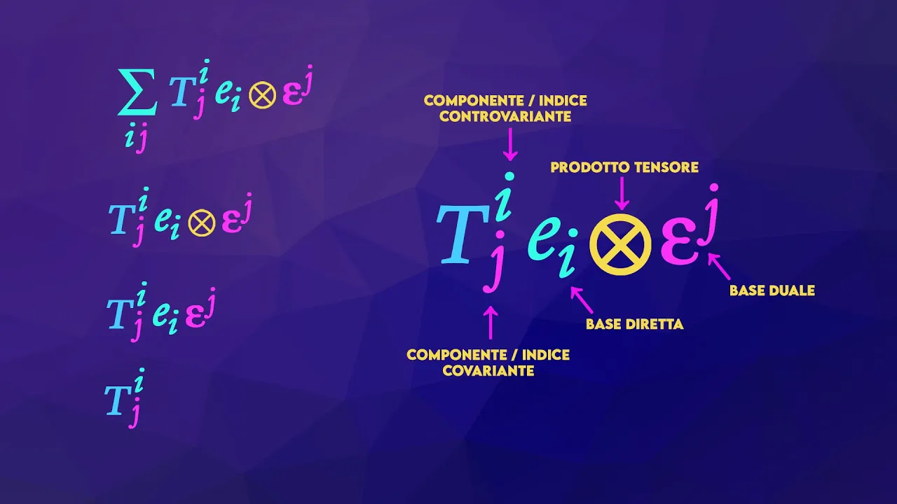
[00:15:20]other tangent vectors are built up using linear combinations of these four basis vectors for example the four velocity vector which used to be defined as d s by d tau where tau is the proper time is now defined as d by d tau and we can use multi-variable chain rule to write this as a linear combination of our four space-time basis vectors so from now on we are going to think of derivative operators as actual vectors and we might write the basis vectors for the tangent spaces using any of these three notations we might use the traditional partial derivative notation or the e basis vector notation or this new partial derivative notation here all of these mean the same thing these are all derivative operators that are also basis vectors the next challenge for intrinsic geometry on manifolds is understanding how vectors change across a manifold in other words we need to understand how to take derivatives of vectors in a vector field in relativity 105 part e i showed how to do this for flat space time using the covariant derivative we just expanded the vector as a linear combination and then used product rule to take the derivatives of both the components and the basis vectors we then expand the derivatives of the basis vectors with respect to lambda using multivariable chain rule and we get linear combinations of the basis vector derivatives with respect to coordinate variables we then once again expand the basis vector derivatives with respect to coordinate variables as linear combinations of basis vectors where the coefficients in the linear combinations are the christophel symbols represented by the capital gammas we get a lot of terms but we can write them compactly as a summation where each component of the vector dv by d lambda has a component derivative term and several christophel symbol terms so i'm going to spend some time talking about covariant derivative notation because the notation can be pretty confusing when i write d by d lambda of v this is taking the covariant derivative of the vector field v in the direction of some curve given by lambda on manifolds a more common notation for the same thing is to write the covariant derivative using the nabla symbol with a subscript vector to indicate the direction of the derivative so here the direction vector subscript is d by d lambda if we said that d by d lambda and w are just two different names for the same vector we could also write this covariant derivative as nabla sub w of v so let's try getting used to this new notation when we take the covariant derivative in a direction that's given by a linear combination of derivative operators we just apply each derivative direction individually and put the scalars out in front this is also true with the nabla notation when the direction vector is a linear combination we just apply the derivative of each direction independently and put the scalars out in front when we take the derivative of a sum of vector fields v and v we just apply the derivative to each one and add the results the same is true in the nabla notation if we have the derivative of a scalar times a vector we just use product rule to get a sum of two terms one with the derivative of the scalar and one with the derivative of the vector again the same is true with nabla notation also in the nabla notation when we have the covariant derivative of a scalar field in some direction this is exactly the same thing as taking the ordinary derivative of a function in that direction now if we ignore this summation with the lambda derivatives we see that the partial derivative of v with respect to x mu is this vector here again we can write this covariant derivative using nabla with the direction vector as a subscript and also recall that the partial derivative with respect to x mu is the same thing as the basis vector e mu so we can write the nabla notation like this the derivative of a vector field in the direction of a basis vector is something that comes up a lot so people have invented special notation for it sometimes in these vector components we write the derivative of the components of v using a subscript comma mu so this subscript comma mu indicates the derivative of the components of v in the x mu direction and sometimes we write this sum of the derivative of the components of v and the christoffel symbol terms together using this notation with a semicolon subscript so this semicolon indicates we are including both the component derivatives and the christophel symbol terms together yet another way of writing this combination is using the nabla with a mu as a subscript this is especially confusing because these two uses of nabla actually refer to different things this term refers to an actual vector whereas this term refers to the components of that vector you can see we're doing a summation with the basis vectors here so these are actually vector components so just to be 100 clear the covariant derivative of a vector field v in some direction is another vector that measures how the vector field v is changing in that direction all of these other notations here measure the components of this vector by measuring the vector using basis vectors so that's enough for the notation now let's talk about actually calculating the covariant derivative on manifolds in order to take derivatives of vectors we need to be able to compare two nearby vectors and see how they are changing over space in flat space time it's easy to compare two vectors that are at different locations we just slide one vector over to the other so that they have the same base point and then we look at the vector difference in curved spaces comparing two vectors at different locations is more challenging it's not immediately obvious how we should move one vector over to the other so that they have the same base point the trick to comparing vectors on a manifold is something called parallel transport to parallel transport a vector along a curve from one point to another we can pretend that the vector is like a sphere or a harpoon in our hand and then we march along the curve keeping the vector as straight as possible so parallel transporting this vector along this curve would look like this we would just be marching forward with the harpoon in our hand and parallel transporting this vector along this curve would look like this we would be walking sideways while holding the harpoon forward so this is how we compare two nearby vectors on a manifold we parallel transport one to the other so that they are in the same tangent space and then we subtract them to see if they are different if we find that the vectors are the exact same after parallel transport then we say that the covariant derivatives of the vectors is zero because the rate of change of the vectors is zero if the vectors are different after parallel transport then the covariant derivative is the difference vector between them which is the rate of change of the vectors so the covariant derivative basically measures how much vectors along a curve deviate away from parallel transport this lets us track how a vector field changes along a curve if a vector field is perfectly parallel transported along a curve the covariant derivative is zero but if the vector field moves away from parallel transport then the covariant derivative would be non-zero now i won't get into the details of why but unfortunately the idea of parallel transport is not enough for us to solve four unique christophel symbols that appear in our covariant derivative we need to specify two additional facts in order to solve for unique christoffle symbols fact number one is that when we parallel transport a pair of vectors we want their lengths and the angle between them to stay the same the fancy name for this property is metric compatibility fact number two is that when we parallel transport a vector basis in different directions by small amounts the vectors should form closed four-sided shapes with each other instead of twisting away and creating a gap the fancy name for this property is torsion free i'm again skipping some details here but the mathematical version of metric compatibility means that when we take the covariant derivative of a dot product we can use product rule over the dot product if we are parallel transporting vectors their covariant derivatives will go to zero and with the metric compatibility property this means that the derivative of their dot product will also be zero this ensures that the lengths of vectors and the angle between them remains constant also if we write the covariant derivatives of basis vectors using christophel symbols and write the dot products of the basis vectors as metric tensor components we can rewrite the metric compatibility property like this the mathematical version of torsion free means that the values of the christoffel symbols stay the same when we switch their lower indices this is something that we got for free in flat space time but we need to state this explicitly in curved space time when we combine the metric compatibility property and the torsionfree property we can solve for a unique set of christoffel symbols which means that we have a unique covariant derivative we can prove this by writing three separate copies of the metric compatibility property using the same indices each time but just shuffled around in each case now because the torsionfree property says that christophel symbols with swapped lower indices are the same and also taking into account that we can swap the lower indices of the metric tensor since the dot product works the same way forwards and backwards these red terms are equal these blue terms are equal and these green terms are equal if we add the first two equations and subtract the third the blue terms cancel the green terms cancel and the red terms add together so we end up with this formula for solving for unique chrosofl symbols we can isolate the christophel symbols on one side if we divide both sides by 2 and sum on both sides with the inverse metric tensor the inverse metric tensor is like the inverse matrix of the metric tensor and it sums with the metric tensor to give us a chronicler delta this covariant derivative that is metric compatible and also torsion free is called the levy chevita connection and you might also see the christophel symbols go by the name of connection coefficients in other sources because it connects different tangent spaces on a manifold by giving us a way to compare vectors in different tangent spaces the last thing i'll mention in this video is geodesics if you recall from relativity 105 f a geodesic was the space-time path a particle traveled along when no forces were acting on it these are just the paths where a particle's for acceleration vector or the second derivative of four position with respect to proper time is zero and if we change the proper time parameter to a generic path parameter lambda this definition also includes the paths of light which are light-like geodesics where proper time is always zero this is called the geodesic equation on curved manifolds the geodesic equation is the exact same except we remove the four position vector and use the derivative operators themselves as tangent vectors the geodesic equation says that the covariant derivative of a vector in the direction of itself is zero in other words it means that a vector is being parallel transported parallel to itself on a sphere parallel transporting a vector parallel to itself would look like this the resulting path is basically the straightest possible path that can be walked along on a curved surface now this is the geodesic equation in its more abstract form which doesn't depend on the coordinate system but the geodesic equation is more useful in its coordinate form so that we can do real calculations we can go from the abstract form to the coordinate form just by writing vectors in terms of a basis and taking their covariance derivative we start with the covariant derivative of v in the direction of v then we expand each v as a linear combination of the basis vectors since the direction input of the covariant derivative is linear we can pull the coefficients outside then we can use product rule on this product to get some terms with the derivative of the components and other terms with the derivatives of the basis vectors now the covariant derivative of component numbers is just the partial derivative and for the covariant derivative of basis vectors we can write the result using a linear combination with the christopher symbols being the coefficients now i'm going to relabel this summation index nu as sigma since we're always allowed to relabel summation indices then i'm going to factor out the e sigma basis vector on the right and then distribute the v mu components on the left and the result is the component version of the geodesic equation now if i treat the vector v as d by d lambda which is the tangent vector along a curve parameterized by lambda then the components of v are just the derivatives of the coordinate variables with respect to lambda and so the geodesic equation looks like this now we can take this summation of derivatives and use multi-variable chain rule in reverse to collapse it to a single derivative with respect to lambda and this becomes a second derivative with respect to lambda now since all of this is equal to the zero vector the components of this vector must all be equal to zero this gives us the component form of the geodesic equation showing all the components equal to zero we'll see later that geodesics that result from parallel transporting a time-like vector with positive squared length along itself will give us the world lines of massive particles in free fall which are only affected by gravity and no forces these time-like geodesics have the longest possible proper time between two events all other paths between the two events that are not geodesics will have a shorter proper time as we've seen in the twin paradox where the twin that forces themselves away from a geodesic to change direction has the smaller proper time also geodesics from light like vectors with zero squared lengths give us the world lines of massless particles like light beams so to summarize this video we said that the equivalence principle means gravity is only detectable in large regions of space-time in small regions of space-time gravity is not detectable this means that the curved space time of general relativity simplifies to the flat space time of special relativity in small regions of space-time this means that space-time is a manifold a curved space that is locally flat specifically it is a pseudo-romanian manifold because each point on the manifold has a metric that can measure vectors that have a positive zero or negative squared length even though we can't use position vectors on a manifold we can still define tangent vectors in the tangent spaces at each point we now treat derivative operators along curves as vectors because they point in a given direction and we can add and scale them together in linear combinations just like vectors we learned parallel transport means carrying a vector along a path while holding it as straight as possible the covariant derivative or levychuvida connection measures how much a vector deviates away from parallel transport along a path and a geodesic curve is one that we get when we parallel transport a vector along itself which results in the straightest possible path on a manifold so again i suspect a lot of people watching this video are going to feel like i covered a lot of content really quickly and will find a lot of this math really confusing all this stuff about manifolds and covariant derivatives is the hardest part of general relativity and i think it requires a few hours of lectures and examples to fully understand it so before moving on i'd strongly encourage you to look at the video links in the description to my tensor calculus playlist and watch and work through the examples i give for geodesics and covariant derivatives on the sphere to understand the ideas better once you understand these things on the two-dimensional sphere it should be less hard to generalize it to the four-dimensional space-time in the next video we're going to introduce the riemann and reache curvature tensors which help us measure the curvature of space-time