Analytical Mechanics: Lagrangian & Hamiltonian Dynamics

Learning Goal: Mastering Classical Analytical Mechanics: From the Principle of Least Action to Lagrangian and Hamiltonian Dynamics. This curriculum transitions you from standard vector-based Newtonian physics to the more powerful, energy-based frameworks of analytical mechanics. You will learn to formulate mathematical descriptions of highly complex, constrained systems, identify hidden conservation laws through the lens of symmetry, and explore the deep geometric properties of phase space.

• Prerequisites: Multivariable Calculus (partial derivatives, path integration), introductory linear algebra, and basic Newtonian mechanics (forces, kinematics, Newton's laws of motion).
• Estimated Total Study Time: 28 Hours

---

Module 1: Mathematical Foundations: Calculus of Variations

Before analyzing physics using energies instead of forces, you must master the mathematical language of optimization: the calculus of variations. This module introduces the concept of functionals—functions of functions—and derives the fundamental Euler-Lagrange equation which finds paths of stationary action.

Recommended Video 1: Derivation of the Euler-Lagrange Equation | Calculus of Variations

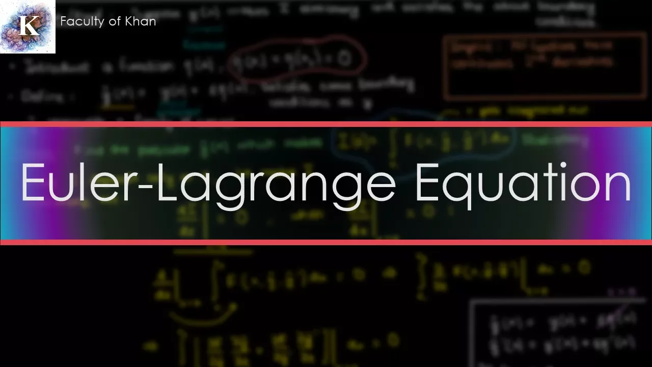
Why this video: This video provides a mathematically clean, step-by-step derivation of the Euler-Lagrange equation. By introducing a variation parameter $\epsilon$ and an arbitrary boundary-vanishing function $\eta(x)$, it clearly demonstrates how extremizing a functional boils down to solving a differential equation. It is the perfect starting point to demystify the calculus of variations.

Knowledge Checkpoint:

• Understand how a functional differs from a standard multivariable function.
• State the definition of the variation function $\eta(x)$ and why it must vanish at the boundary endpoints.
• Walk through the integration-by-parts step that transitions the integrand from containing $\eta'(x)$ to isolating $\eta(x)$.

Recommended Video 2: 02: Fundamentals part2, Generalized coordinates

Why this video: To map physical spaces to optimization frameworks, you must abandon rigid Cartesian coordinate systems. This rigorous academic lecture explains how generalized coordinates ($q_i$) represent the true, unconstrained degrees of freedom of a system. It provides the geometric foundation needed to construct Lagrangians for arbitrary mechanical systems.

Knowledge Checkpoint:

• Define what makes a set of coordinates "generalized."
• Calculate the number of degrees of freedom for a system of $N$ particles with $k$ holonomic constraints.
• Express velocity transformations from Cartesian coordinate derivatives to generalized coordinate derivatives using the chain rule.

Recommended Video 3: The Calculus of Variations and the Euler-Lagrange Equation

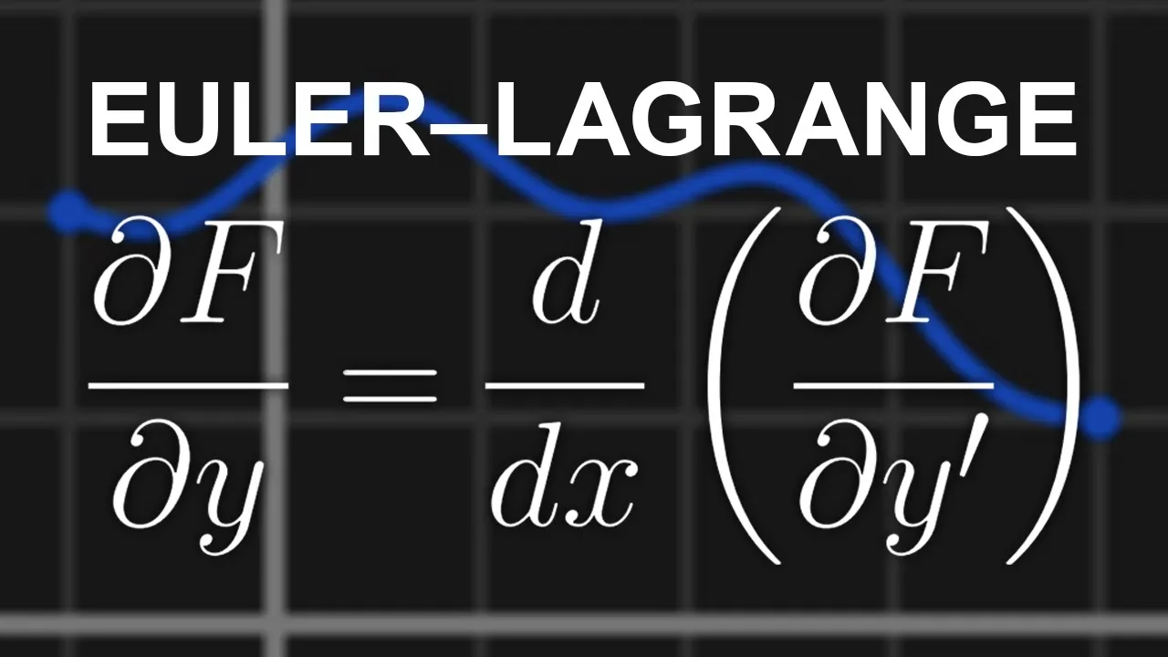
Why this video: This video serves as an excellent visual and conceptual reinforcement of the mathematical tools learned in this module. It contrasts normal single-variable optimization with functional optimization, reinforcing the geometric intuition of finding a stationary "path" through configuration space.

Knowledge Checkpoint:

• Define the mathematical form of a functional $J[y]$.
• Explain why the derivative of the functional with respect to the variation parameter must equal zero ($\frac{dJ}{d\epsilon}\big|_{\epsilon=0} = 0$) at the extremum.

---

Module 2: Newtonian Limits & Constraint Dynamics

While Newton's second law ($F=ma$) is conceptually simple, it becomes highly impractical when systems are subject to constraints (e.g., a bead sliding on a shaped wire or a double pendulum). This module explores why Newtonian mechanics struggles in these scenarios, defines the classifications of constraints, and introduces D'Alembert's Principle of virtual work to systematically bypass constraint forces.

Recommended Video 1: Constraints and generalized coordinates

Why this video: This video details the mechanical limits of Newtonian vector mechanics and explains how constraints restrict physical motions. It introduces the vital distinction between holonomic constraints (which can be written as algebraic equations relating coordinates) and non-holonomic constraints (which involve velocities or inequalities, like rolling without slipping).

Knowledge Checkpoint:

• Differentiate between holonomic and non-holonomic constraints with physical examples.
• Explain how a constraint equation mathematically reduces the dimensionality of the system's configuration space.
• Identify why constraint forces (like tension or normal force) are difficult to solve directly in Newtonian mechanics.

Recommended Video 2: D'Alembert's principle | Explained

Why this video: D'Alembert's principle bridges Newtonian mechanics and analytical mechanics. This video intuitively explains how d'Alembert transformed a dynamic problem of motion into a static problem of equilibrium by introducing the concept of "inertial forces" ($-\dot{p}$) coupled with virtual displacements.

Knowledge Checkpoint:

• Define virtual displacement and explain how it differs from real, differential displacement ($dt > 0$).
• Explain why the net virtual work done by forces of constraint is equal to zero for rigid, holonomic constraints.
• Write down the symbolic expression for D'Alembert's principle.

Recommended Video 3: D' Alemberts Principle | Dynamics | Engineering Mechanics

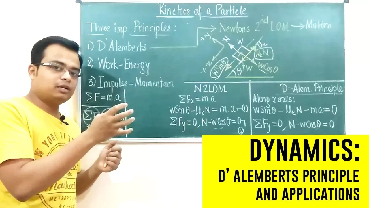
Why this video: To gain practical problem-solving experience, this video walks through physical applications of D'Alembert's Principle. It provides engineering and physics students with a clear view of how virtual static equilibrium simplifies actual dynamical systems under constraints.

Knowledge Checkpoint:

• Set up a dynamic force balance equation using D'Alembert's reverse-inertia formulation.
• Banish constraint forces from active work equations by applying virtual displacements perpendicular to those constraints.

💡 Curriculum Gap Alert: Finding high-quality, deeply rigorous video proofs of the derivation of Lagrange's equations directly from D'Alembert's principle can be challenging online. To master this transition, it is highly recommended to complement this module by reviewing Chapter 1 of Classical Mechanics by Herbert Goldstein. Focus on how the expression $\sum (F_i - \dot{p}_i) \cdot \delta r_i = 0$ is converted into generalized coordinates to yield the Euler-Lagrange equations.

---

Module 3: The Principle of Least Action & Lagrangian Mechanics

We now arrive at the heart of analytical mechanics: Hamilton's Principle of Least Action. Instead of tracking instantaneous vector forces, we define a single scalar quantity—the Lagrangian ($L = T - V$, kinetic minus potential energy)—and state that a system's true path through time is the one that minimizes (makes stationary) the integrated action.

Recommended Video 1: Euler-Lagrange equation explained intuitively - Lagrangian Mechanics

Why this video: This highly visual and intuitive explanation is legendary for making the Principle of Least Action accessible. It animates how nature "tests" adjacent paths in configuration space and shows that the path physically taken is the one where the total action $S = \int L \, dt$ does not change to first order.

Knowledge Checkpoint:

• Define the Lagrangian $L$ and the Action functional $S$.
• Explain physically why a path that minimizes action balances kinetic and potential energy over time.
• Describe how changing the starting or ending time changes the action calculation.

Recommended Video 2: Lagrangian and Hamiltonian Mechanics in Under 20 Minutes: Physics Mini Lesson

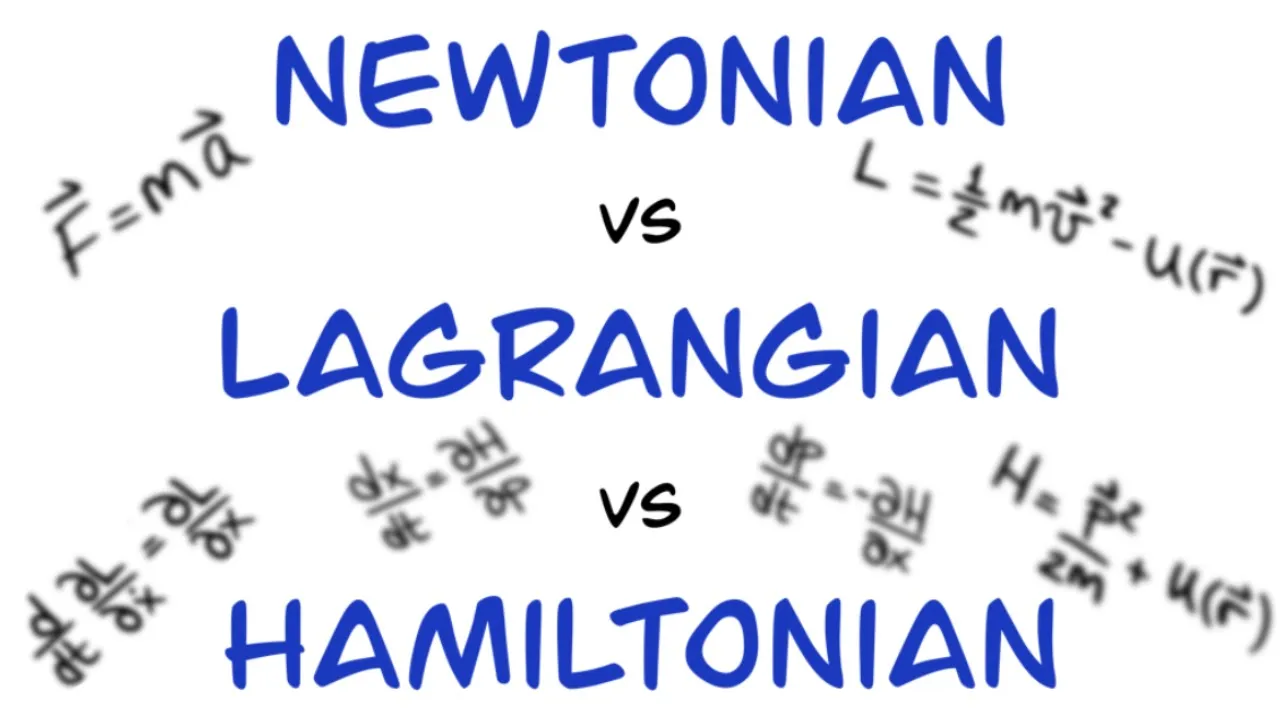
Why this video: This concise, high-density mini-lesson acts as a bridge between the mathematical derivation and its direct physical implementation. It walks through how to construct a simple pendulum's Lagrangian and feed it into the Euler-Lagrange equation to easily obtain its equations of motion.

Knowledge Checkpoint:

• Write down the kinetic energy $T$ and potential energy $V$ of a simple pendulum in terms of the generalized coordinate $\theta$ and its velocity $\dot{\theta}$.
• Compute the partial derivatives $\frac{\partial L}{\partial \theta}$ and $\frac{\partial L}{\partial \dot{\theta}}$ for the pendulum system.
• Apply the Euler-Lagrange formula to write the final equation of motion.

Recommended Video 3: Physics 68 Lagrangian Mechanics (2 of 25) Why Does the Lagrangian Equation Work?

Why this video: Michel van Biezen provides clear, structured academic board work. This video illustrates why the mathematical architecture of Lagrangian mechanics naturally yields Newton's second law when applied to simple, unconstrained systems like a particle in free fall. It builds confidence in the equivalence of these two frameworks.

Knowledge Checkpoint:

• Prove that for a 1D conservative system, $\frac{\partial L}{\partial x}$ represents the force $F_x$, and $\frac{d}{dt}\left(\frac{\partial L}{\partial \dot{x}}\right)$ represents mass times acceleration ($ma_x$).
• State the physical units of Action.

---

Module 4: Solving Systems & Noether's Theorem

Lagrangian mechanics shines brightest when solving complex, multi-body systems and unveiling deep conservation laws. This module walks you through solving the chaotic double pendulum and introduces Emmy Noether's revolutionary theorem, which connects continuous coordinate symmetries directly to physical conservation laws (like energy, momentum, and angular momentum).

Recommended Video 1: The Biggest Misconception in Physics

Why this video: This highly engaging Veritasium video is a phenomenal introduction to Emmy Noether and her monumental theorem. It explains how symmetries of the Lagrangian under continuous transformations guarantee the existence of conserved quantities, completely changing how physicists understand the laws of nature.

Knowledge Checkpoint:

• Explain what a "continuous symmetry" is in a physical system.
• State which conservation laws correspond to time translation symmetry, spatial translation symmetry, and rotational symmetry.
• Explain why conservation laws are not just arbitrary empirical observations, but mathematical consequences of symmetry.

Recommended Video 2: Lagrangian Mechanics and the Double Pendulum

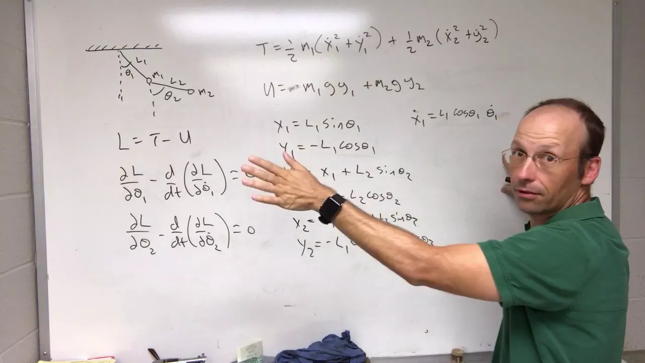
Why this video: The double pendulum is the classic benchmark of analytical mechanics. This video demonstrates the process of setting up the Lagrangian for this complex system. It shows how handling constraint forces Newtonian mechanics, whereas Lagrangian mechanics solves it through pure coordinate-algebra and energy relationships.

Knowledge Checkpoint:

• Express the coordinates ($x_1, y_1$) and ($x_2, y_2$) of both pendulum masses in terms of the two angles $\theta_1$ and $\theta_2$.
• Set up the full kinetic energy function $T$, identifying the complex cross-terms that link $\dot{\theta}_1$ and $\dot{\theta}_2$.
• Recognize why analytical solutions are impossible and numerical approximations are required for the double pendulum.

Recommended Video 3: Double Pendulum Simulation in Processing: A Step-by-Step Coding Challenge

Why this video: To make analytical mechanics actionable, this coding challenge translates the derived differential equations of motion for the double pendulum into a live computer simulation. It connects advanced math directly to physical, chaotic behavior on screen.

Knowledge Checkpoint:

• Identify how the analytical expressions for angular accelerations ($\ddot{\theta}_1, \ddot{\theta}_2$) are structured in a simulation loop.
• Explain how numerical integration techniques (like Euler or Runge-Kutta) update positions and velocities over small time increments ($dt$).

Recommended Video 4: Noether's Theorem Explained (Part 1/6) - Introduction

Why this video: This academic video provides a rigorous mathematical introduction to Noether's theorem. It explicitly calculates how a small coordinate shift $\delta q$ leaves the action invariant, proving how the conservation equation mathematically falls out of the Euler-Lagrange equations.

Knowledge Checkpoint:

• Define the conjugate momentum $p_i$ as a partial derivative of the Lagrangian.
• Prove mathematically that if a Lagrangian does not explicitly depend on a coordinate $q_i$ (a cyclic coordinate), its conjugate momentum $p_i$ is conserved over time.

---

Module 5: Hamiltonian Dynamics & Phase Space

We now pivot from the Lagrangian description ($2N$-dimensional configuration space governed by $N$ second-order differential equations of position and velocity) to the Hamiltonian formulation. By applying a Legendre transformation, we construct the Hamiltonian ($H(q,p)$) based on position and momentum. This results in $2N$ coupled, first-order canonical equations, opening up a geometric interpretation of physics in phase space.

Recommended Video 1: Lagrangian vs Hamiltonian Mechanics

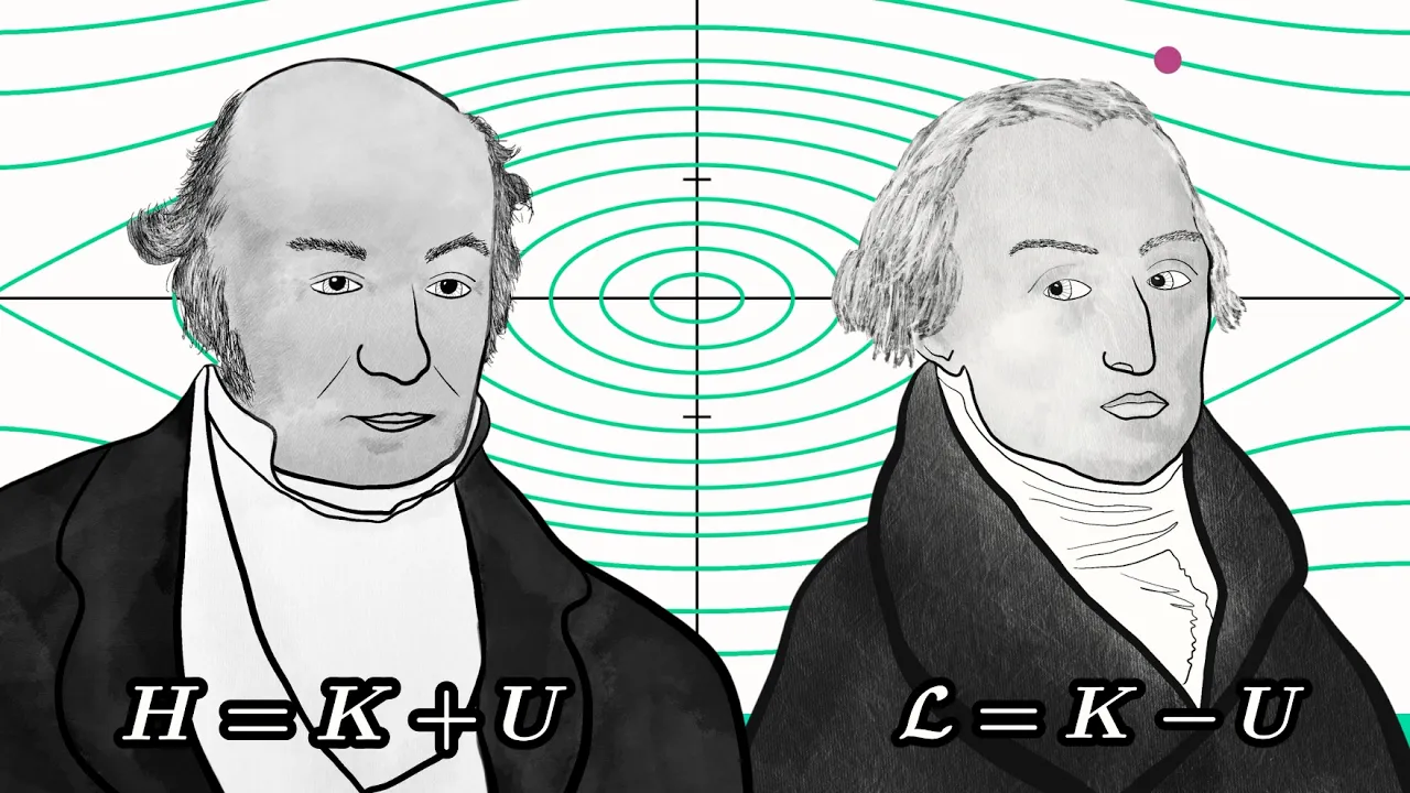
Why this video: This video provides a deep comparative breakdown of both formulations. It details why we transition to Hamiltonian mechanics (the gateway to quantum mechanics and statistical mechanics) and explains how changing the independent variable from velocity ($\dot{q}$) to momentum ($p$) alters the mathematical landscape.

Knowledge Checkpoint:

• Contrast the state-space of Lagrangian mechanics (configuration space + velocities) with that of Hamiltonian mechanics (phase space).
• State why having first-order differential equations is advantageous over second-order differential equations.
• Explain how the Hamiltonian $H$ relates to the total energy of a system in static coordinate frameworks.

Recommended Video 2: Legendre Transformation explained (with Animation)

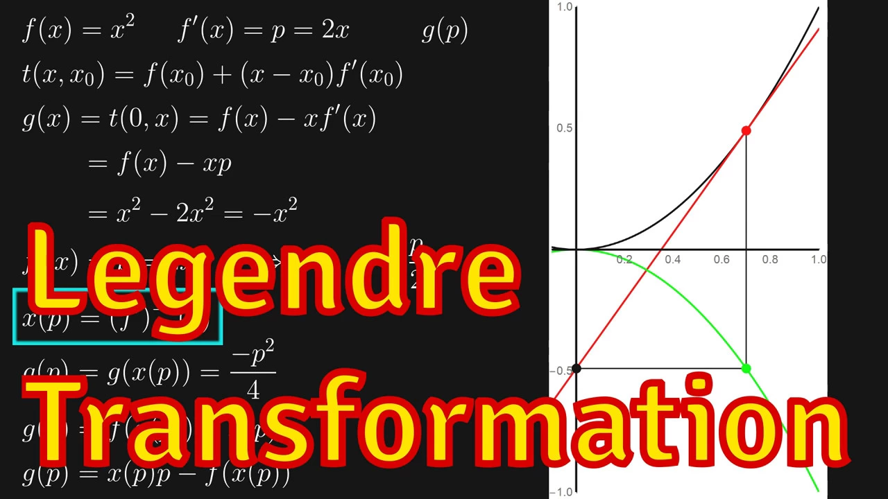
Why this video: The Legendre transform is the crucial mathematical tool used to convert a Lagrangian $L(q, \dot{q})$ into a Hamiltonian $H(q,p)$. This video provides an elegant animated explanation of how the Legendre transform converts a function of a variable into an equivalent function of its derivative (slope) without losing any physical information.

Knowledge Checkpoint:

• Explain how a function can be represented as an envelope of tangent lines instead of individual coordinate points.
• Write down the algebraic equation of the Legendre transform of $f(x)$ to $g(p)$, where $p = f'(x)$.
• Show how $H = \sum p_i \dot{q}_i - L$ is a direct application of this transform.

💡 Curriculum Gap Alert: While this visual explanation of the Legendre transform is excellent, it is highly recommended to study its physical application in thermodynamics (transforming Internal Energy to Helmholtz/Gibbs Free Energy) to gain a complete, multi-disciplinary intuition.

Recommended Video 3: Derivation of Hamilton's Equations of Motion | Classical Mechanics

Why this video: This concise video walks through the derivation of Hamilton's canonical equations of motion. By taking the total differential of $H(q,p) = p \dot{q} - L(q, \dot{q})$ and comparing the mathematical coefficients of $dq$ and $dp$, it cleanly extracts the two coupled dynamical equations.

Knowledge Checkpoint:

• Write down Hamilton's Equations: $\dot{q}_i = \frac{\partial H}{\partial p_i}$ and $\dot{p}_i = -\frac{\partial H}{\partial q_i}$.
• Account for the physical origin of the negative sign in the equation for $\dot{p}_i$.

Recommended Video 4: Lecture 1 | The Theoretical Minimum

Why this video: Presented by Leonard Susskind, this introductory snippet of "The Theoretical Minimum" provides the conceptual foundation of Phase Space. It explains how any physical state of a system is represented as a single point in a multidimensional space of positions and momenta, and how time evolution draws a deterministic, non-intersecting trajectory through this space.

Knowledge Checkpoint:

• Explain why trajectories in classical phase space can never cross each other.
• Define the dimension of phase space for a system with $N$ independent particles moving in 3D space.

---

Module 6: Advanced Topics: Poisson Brackets & Canonical Transformations

This final module explores the deeper algebraic structures of classical mechanics. You will learn about Poisson Brackets, which act as the classical precursor to the quantum mechanical commutator. You will also study canonical transformations (coordinate changes that preserve the form of Hamilton's equations) and catch a glimpse of the Hamilton-Jacobi theory, which treats motion as a continuous transformation of coordinates.

Recommended Video 1: Classical Mechanics | Lecture 8

Why this video: In this advanced lecture segment from Stanford, the concept of Poisson brackets is formally introduced. It shows how the time derivative of any physical quantity $f(q,p,t)$ can be elegant written in terms of its Poisson bracket with the Hamiltonian: $\dot{f} = \{f, H\} + \frac{\partial f}{\partial t}$.

Knowledge Checkpoint:

• Write down the mathematical definition of the Poisson Bracket $\{f,g\}$ of two functions of phase space.
• Prove the fundamental Poisson brackets: $\{q_i, q_j\} = 0$, $\{p_i, p_j\} = 0$, and $\{q_i, p_j\} = \delta_{ij}$.
• Explain how a quantity $f$ is conserved if its Poisson bracket with the Hamiltonian $\{f, H\} = 0$ (assuming no explicit time dependence).

Recommended Video 2: Classical Mechanics - Canonical Transformations : What’s a Canonical Transformation

Why this video: This lecture explains canonical transformations: coordinate transformations $(q,p) \rightarrow (Q,P)$ that preserve the exact form of Hamilton's equations. This mathematical structure allows physicists to simplify highly complex coordinate geometries into trivial linear systems.

Knowledge Checkpoint:

• Define the condition for a coordinate transformation to be "canonical."
• Describe the role of a Generating Function ($F_1, F_2, F_3, F_4$) in executing canonical transformations.
• Explain how Poisson brackets are invariant under canonical transformations (i.e., $\{Q_i, P_j\}_{q,p} = \delta_{ij}$).

Recommended Video 3: Method of Separation of Variables to solve the Hamilton-Jacobi equation

Why this video: This practical, mathematically focused video introduces the Hamilton-Jacobi equation. By transforming coordinates such that the new Hamiltonian is identically zero, all new positions and momenta become constants of motion. The video shows how to solve this partial differential equation using the separation of variables method.

Knowledge Checkpoint:

• State the core goal of the Hamilton-Jacobi theory.
• Write down the Hamilton-Jacobi equation for Hamilton's principal function $S(q, \alpha, t)$.
• Explain how solving for $S$ directly generates the paths of motion for the system.

---

Course Map

---

Key People Index

• Joseph-Louis Lagrange (1736–1813): Italian-French mathematician and astronomer. He revolutionized mechanics by publishing Mécanique analytique (1788), proving that mechanics could be formulated purely using scalar energy algebraic functions without any geometry or force vectors.
• William Rowan Hamilton (1805–1865): Irish mathematician who formulated the principle of least action (Hamilton's Principle) and reformulates mechanics in terms of conjugate momentum variables, providing the mathematical architecture for quantum theory.
• Emmy Noether (1882–1935): Landmark German mathematician. Described by Einstein as the most significant creative mathematical genius since the higher education of women began. She discovered and proved Noether's Theorem, fundamentally uniting physics with coordinate symmetry.
• Jean le Rond d'Alembert (1717–1783): French mathematician and physicist. He pioneered the reduction of dynamic problems to statics using virtual displacements and inertial forces.

---

Final Self-Assessment

Test your mastery of classical analytical mechanics by verifying your ability to explain or perform the following tasks:

• 1. Derive the Euler-Lagrange equation from the starting condition that the first variation of the action is zero ($\delta S = 0$).
• 2. Classify a physical constraint (e.g., a rolling disk, a pendulum with variable string length) as holonomic, non-holonomic, scleronomous, or rheonomous.
• 3. Construct the virtual work equation for a constrained system and explain why constraint forces disappear from the formulation.
• 4. Correctly write down the Lagrangian ($L = T - V$) for a multi-degree of freedom system (like a double pendulum or a particle on a rotating hoop) using generalized coordinates.
• 5. State Noether's Theorem and mathematically prove that if $\frac{\partial L}{\partial q_i} = 0$, then the conjugate momentum $p_i = \frac{\partial L}{\partial \dot{q}_i}$ must be a constant of motion.
• 6. Mathematically perform a Legendre transform on a simple function of one variable, converting it from $f(x)$ to $g(p)$.
• 7. Write down Hamilton's canonical equations of motion and derive them directly from the Hamiltonian $H = \sum p_i \dot{q}_i - L$.
• 8. Explain the concept of Phase Space and prove why the trajectory of a classical, deterministic system can never intersect itself.
• 9. Calculate the Poisson bracket of two given functions of coordinates and momenta, and use it to determine if a given dynamical quantity is conserved under time evolution.
• 10. Verify whether a given coordinate transformation $(q,p) \rightarrow (Q,P)$ is canonical by calculating its fundamental Poisson brackets.