







![ASMR Boring Math Lecture To Put You To Sleep - Differential Equations and Integration [Request]](https://i.ytimg.com/vi/dwzs1Azs848/maxresdefault.jpg)











![[물리를 이해하며 함께하는 수학, 무리함수] 라그랑주 역학과 뉴턴 역학, 최소강하곡선 문제](https://i.ytimg.com/vi/TfS9uq6e1i4/maxresdefault.jpg)




The calculus of variations extends optimization from functions to functionals, which map functions to real numbers; to find the stationary points of a functional J[y] = ∫F(x, y, y')dx between two fixed points, we consider small variations ȳ = y + εη(x) with η(0) = η(1) = 0, apply Leibniz's rule and integration by parts, and derive the Euler-Lagrange equation ∂F/∂y - d/dx(∂F/∂y') = 0, which characterizes the extremal curves that minimize or maximize the functional.
Calculus of Variations & Euler-Lagrange Equation Derivation
Added:Multivariable calculus, specifically partial derivatives, the chain rule, and the technique of integration by parts.
Fundamental concepts of optimization in single-variable calculus, such as locating local extrema by finding where a derivative equals zero.
Basic proficiency in solving first-order and second-order Ordinary Differential Equations (ODEs).
Familiarity with Newtonian mechanics (specifically position, velocity, kinetic energy, and potential energy) to understand the physical context of these mathematical tools.
Lagrangian Mechanics and Hamilton's Principle of Least Action to reformulate classical mechanics using kinetic and potential energy.
Constrained variational problems, such as the Isoperimetric Problem, utilizing Lagrange multipliers for functionals.
Hamiltonian Mechanics, which transitions from Lagrangian configuration space to phase space via Legendre transformations.
Advanced applications in differential geometry (finding geodesics on arbitrary curved manifolds) and optimal control theory (such as Pontryagin's Maximum Principle).
143.2K views3.4Klikes6:02Original Release: 2019-02-22
Hey everyone, in today's video I want to provide an introduction to calculus of Variations and show how we derive the Euler Lagrange equation and hopefully give some visual intuition for it.
But we need to start with something that you might find a bit more familiar, optimizing single variable functions.
from single variable calculus you may recall how we find the local maxima and minima of functions given some function f(x).
A local minimum or maximum can occur at any point where the slope of its tangent line df/dx is equal to 0 This should make intuitive sense since we're just saying that a step in any direction will basically take you nowhere.
This is a very key idea: at a local minimum or maximum, any small change in your input to the function will return a value further away in the same direction from your previous output. In calculus of variations, we're not concerned with finding fixed points of functions, but rather fix points of functionals.
The types of functions we had just looked at had a very specific set of properties They had a domain and range of the real numbers Essentially you can kind of think of these functions like a machine you put a real number in and you get a real number out.
Functionals are a little different though, with functionals you input a function and get a real number out. To help distinguish between functions and functionals, we typically put their inputs around square brackets as opposed to parentheses.
There's a crucial change happening here, and I hope you don't miss it: Since a functional takes a function as an input our value can depend on any function of x y and its derivatives.
More information is fundamentally encoded in it.
We're going to spend the remainder of this video looking at a specific form of functional J[y(x)] Equals the integral of F(x, y, y') dx. If we're given a curve y, F just becomes a function in terms of x and when we integrate over it, we're essentially summing all of its values over the curve y(x). While this may seem a little pointless now it ends up being a very important idea. An example you may be familiar with is finding the arc length of a curve.
We can write the arc length as the integral of the square root of 1 plus (y')^2.
Notice that this perfectly fits the form of J of y. Another problem you may be familiar with is the Brachistochrone problem.
You can write the time it takes to roll down a function as this integral. Another important example is found in Lagrangian Mechanics.
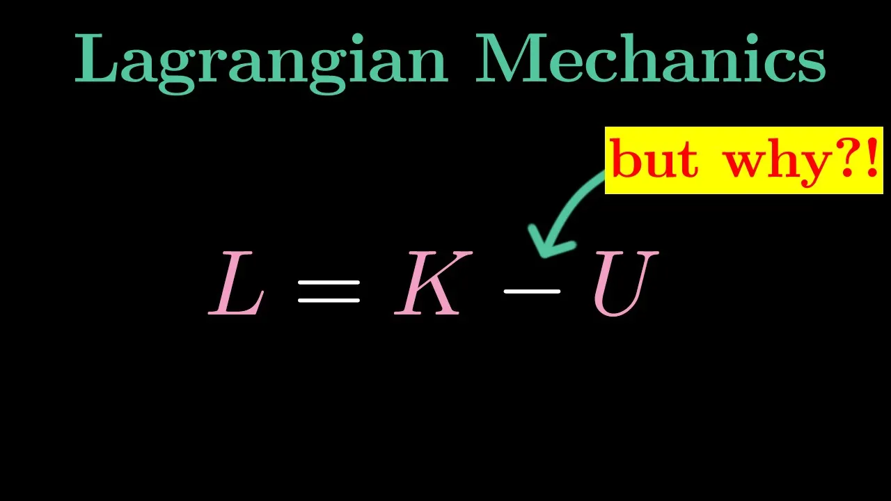
Lagrange managed to show that a particle will take a path where the integral of its kinetic energy minus its potential energy - commonly called the Lagrangian - is the lowest. This also fits the form of J[y].
Now that you've gotten a sense for functionals, Let's take a look at the central problem of the calculus of variations. For two points A(x0, y0), and B(x1, y1), there are an infinite number of curves that pass through them. What we want to do is find the curve That is the stationary point of J[y].
Fundamentally, we're finding a curve between A and B that minimizes the integral of F over it.
We're going to solve this in a similar way to how we solve the one dimensional problem.
We're going to consider what happens when we add a small change to our input, but in this case any small change to our input would be a function.
Let's say that y is an extremal of J[y].
We let y bar equal y plus epsilon times eta(x). Here epsilon times eta is the small change in the function. To ensure that y bar still fits our boundary conditions, we need to let eta(x0) equal eta(x1) equal zero.
Notice that J[y bar] is now just a function of epsilon, J(epsilon). Since epsilon equals zero is an extremal of J, we know that J'(epsilon) at epsilon equals zero equals zero.
Let's pay attention to simplifying dJ/d(epsilon). From Leibniz's rule, we can rewrite this as the integral of partial F partial epsilon from x0 to x1 dx.
Using the multivariable chain rule, partial F partial epsilon becomes partial F partial y bar times partial y bar partial epsilon plus partial F partial y bar prime times partial y bar prime partial epsilon.
Referring back to our definition of y bar, we can simplify this again as partial F partial y bar times eta plus partial F partial y bar prime times eta prime. I now want to draw your attention to this term.
Partial F partial y bar prime times eta Prime. We can use integration by parts to break up this integral even further.
We let u equal partial F partial y bar prime and dv equal eta prime dx.
then du equals d on dx of partial F partial y bar prime and v equals the integral of eta prime, which is just eta. By the rules of integration by parts, we can then rewrite this integral as partial F partial y bar prime times eta from x0 to x1 minus the integral of eta times d on dx of partial F partial y bar prime dx from x0 to x1.
Notice that the first term becomes 0 since eta of x0 and eta of x1 both equal 0.
If you plug this back into our original integral and factor out the eta in both terms, We get the integral of partial F partial y bar minus d on dx partial F partial y bar prime times eta. For our integral to be equal to 0 generally, we need this term to be equal to 0. This leaves us with the Euler-Lagrange equation.
It is arguably one of the most important equations ever, and it completely revolutionized mathematics and physics. As a summary, today we learned what it means to optimize a function, what a functional is and some of their applications, how to optimize a specific type of functional, and hence derived the Euler Lagrange equation.
I don't think I'm quite ready to do a series on calculus variations, but I do plan to do a couple of worked examples with it, so let me know if that's something you'd be interested in. If you have any questions or spotted any mistakes, feel free to leave a comment.
Up Next
7:50
Deriving the Euler-Lagrange Equation | Variational Calculus
@FacultyofKhan
289.9K views•2017-07-17

4:43
Elliptic Curve Cryptography Explained: ECC, ECDSA, ECDH
@PracticalNetworking
28.5K views•2024-10-21

10:44
Fourier Series Introduction: The Big Idea Explained
@DrTrefor
387K views•2021-05-03

6:00
The Mathematical Impossibility of Accurate World Maps
@Vox
23.3M views•2016-12-02
Related Study Plans & Knowledge Roadmaps
Structured learning paths in Mathematics
mathematics
Tensor Calculus: Vectors to Riemann Curvature
01Mathematical Foundations: Linear Algebra & Calculus
02Covectors, Dual Spaces, and Tensor Basics
03The Metric Tensor and Index Gymnastics
+ 2 more learning modules
40h5 modules
Explore Roadmap
mathematics
Gödel's Incompleteness: Logic, Proofs & Limits
01Introduction to Formal Systems & Hilbert's Dream
02Set Theory, Cardinality, and Cantor's Diagonal Argument
03Arithmetization and Gödel Numbering
+ 2 more learning modules
14h5 modules
Explore Roadmap
mathematics
Galois Theory: Fields, Groups & Solvability
01Foundations of Abstract Algebra: Groups & Fields
02Polynomials & Field Extensions
03Splitting Fields & Symmetries
+ 2 more learning modules
24h5 modules
Explore Roadmap
mathematics
Non-Euclidean Geometry: Models & Geodesics
01Euclid's Fifth Postulate and the Birth of New Geometries
02Hyperbolic Space and the Poincaré Disk Model
03Geodesics: Defining Straight Lines in Curved Spaces
+ 2 more learning modules
15h5 modules
Explore Roadmap