

















![23 - Mecánica Teórica [Reformulación del oscilador armónico]](https://i.ytimg.com/vi/Tglf8OYiciU/maxresdefault.jpg)

![26 - Mecánica Teórica [Hamilton-Jacobi vs Schrödinger]](https://i.ytimg.com/vi_webp/F5hMeusKfr0/maxresdefault.webp)



Lagrangian mechanics uses the Lagrangian (kinetic minus potential energy) and the principle of least action to derive equations of motion through the Euler-Lagrange equations, while Hamiltonian mechanics uses the Hamiltonian (total energy) and provides two first-order differential equations through Hamilton's equations; these two formulations are mathematically equivalent and related by the Legendre transform, which converts between generalized coordinates and momenta, enabling a new geometric view of physics through phase space analysis.
Lagrangian vs Hamiltonian Mechanics: The Legendre Transform Link
Added:Familiarity with Lagrangian mechanics, including the Principle of Least Action and the derivation of the Euler-Lagrange equations.
An understanding of generalized coordinates, generalized velocities, and the concept of conjugate (canonical) momentum.
Solid foundations in multivariable calculus, particularly partial derivatives, total differentials, and coordinate transformations.
A basic grasp of Newtonian mechanics, kinetic and potential energy, and classical conservation laws.
Formulating and solving physical systems using Hamilton's canonical equations of motion in phase space.
Exploring Canonical Transformations and Poisson Brackets, which reveal the deeper algebraic structure of Hamiltonian systems.
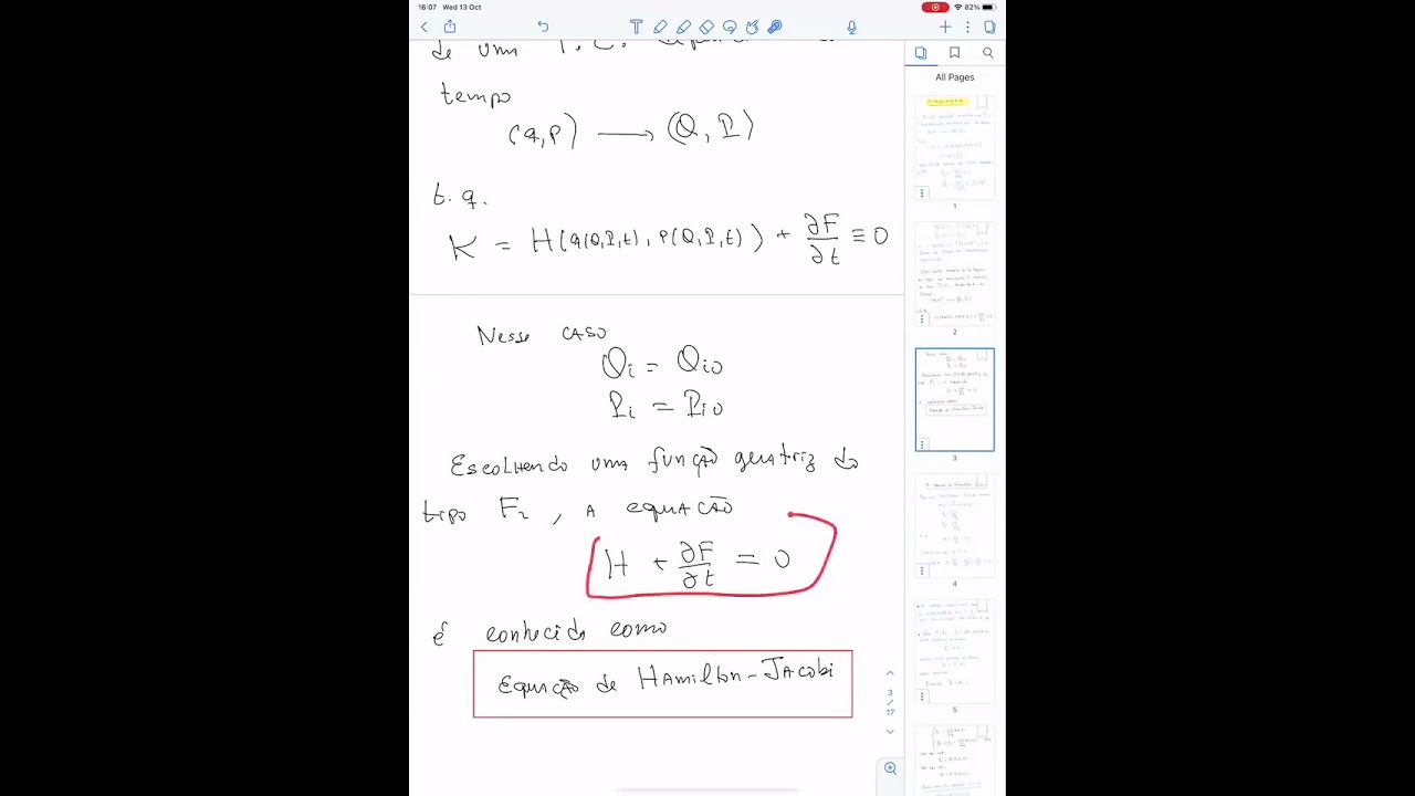
Studying Hamilton-Jacobi Theory, which connects classical trajectory mechanics to wave propagation.
Investigating how Hamiltonian mechanics serves as the mathematical foundation for both Statistical Mechanics and the transition to Quantum Mechanics via canonical quantization.
174K views6.3Klikes20:56Original Release: 2025-09-26
Who invented calculus? Isaac Newton or Gotfrieded Linets? One of the most infamous debates in the history of science. The controversy came to a peak in 1712 with the publication of this manuscript. It contained a collection of letters and papers meant to definitively prove that Isaac Newton was the true inventor of calculus. In his own summary of these events, Newton referred to Linets as a second inventor who has no rights.
Despite Newton receiving sole credit for the next century or so, the modern consensus has changed. Both Newton and Linets are now seen as each having invented calculus completely independently of one another. But there was another controversy between these two intellectual giants that is lesser known yet arguably more important.
Whether physics is best described by a geometric vector approach or an analytic functional approach. It was a controversy so fruitful that it led to the development of three alternative formulations of classical mechanics. the discovery of one of the most foundational principles in all of physics and ultimately produce the right theoretical framework that would make the advent of quantum mechanics possible. My aim with this video is to show you the strength of the analytical approach to physics. The focus will be on these two formulations of mechanics and how they are related to one another.
Along the way, we'll also see that although lrangeian and Hamiltonian mechanics abandons the Newtonian geometric vector approach, an entirely new geometric view of physics emerges.
In a classic book on analytical mechanics, the physicist Cornelius Lantros wrote that linenets is the originator of analytical mechanics which is entirely based on two fundamental scalar quantities. kinetic energy and potential energy. This branch of mechanics inspired by linenets was further developed by two famous mathematical physicists, Joseph Louie Lrange and William Rowan Hamilton.
Incredibly, in both lrangeian and Hamiltonian mechanics, these two scalar quantities contain all the information you need in order to successfully understand the dynamics of any physical system. How is this possible? Let's see how it works with a basic example, the simple pendulum. We'll analyze it by first using Lrange's approach and then Hamilton's. In this model, a ball of mass m is attached by a rod of length r to a fixed support. The rod is massless.
There's no friction and the pendulum is under the influence of gravity.
According to Lrangege, the first thing we need to do is to write down a quantity called the Lrangeian, which equals the kinetic energy minus the potential energy. If you'd like to know where exactly this equation comes from, I made an entire video about it that I've linked below. For now, I'll just briefly summarize it with two points.
First, if you consider a 2D mathematical space where one axis is the kinetic energy and the other axis is the potential energy, the langrian represents the trajectory the system takes in this energy space. Second, there is an important quantity in physics called the action which is defined by taking the integral of the lrangeian over some time span. The principle of least action says that of all possible paths that a particle can take, the one that it will always take is the one that minimizes or rather extremisizes the action. And in order for the action to be extremized, the oiler lrange equations must hold. So if you want to begin with the principle of least action and arrive at the same equations of motion that Newton's second law gives the lrangeian that needs to be plugged in is the one where L= K minus U. I go into detail about all of this in the linked video. So be sure to go check it out after this. Now in order to write down the lrangeian of the simple pendulum we first need to define a coordinate system. We'll call the arklength coordinate S. This is the coordinate that runs along the circumference of the circle traced out by the mass. We'll also define the angle away from the midpoint as theta. By definition of the arc length, these two are related by the equation theta = s r or s = r theta. The kinetic energy is just 12 mass * velocity. And in this coordinate system, the position is given by s. Now since velocity is just the change in position over time, we can express the velocity as the derivative of the position or using Newton's notation as s dot. So kinetic energy is 12 m * s dot squ or equivalently we can use this expression to write the kinetic energy in terms of theta. The potential energy on the other hand is given by mgh where h is the height of the mass above some level that we define to be zero.
Here I'll set up a new coordinate and declare h= 0 as the location of the pivot. So the height of the pendulum is given by r * cosine theta which gives the following for the difference between the kinetic energy and potential energy.
According to lrangee after writing down the lrangeian for a given system we then need to plug it into the oiler lrangee equations for the right hand side we treat theta and theta dot as independent variables. So we take the derivative of l with respect to theta and treat theta dot as a constant. For the left hand side we first treat theta as a constant and take the partial derivative of l with respect to theta dot. Then we take the derivative of the result with respect to time. Setting these two equations equal to each other and cancelling like terms results in one second order differential equation that entirely describes the motion of the system which is the exact same equation you would get if you began with Newton's F= ma vector approach. This differential equation turns out to actually be quite complicated to solve in general and it's mainly due to this sin theta term. But if we restrict ourselves to only considering the special case when theta is small, so the pendulum doesn't move too far away from its equilibrium point, then we can write down a solution. In this case, we employ the so-called small angle approximation and replace sin theta by theta. The solution then turns out to just be cosine or equivalently s.
Okay, let's now consider how to analyze our system using Hamilton's approach.
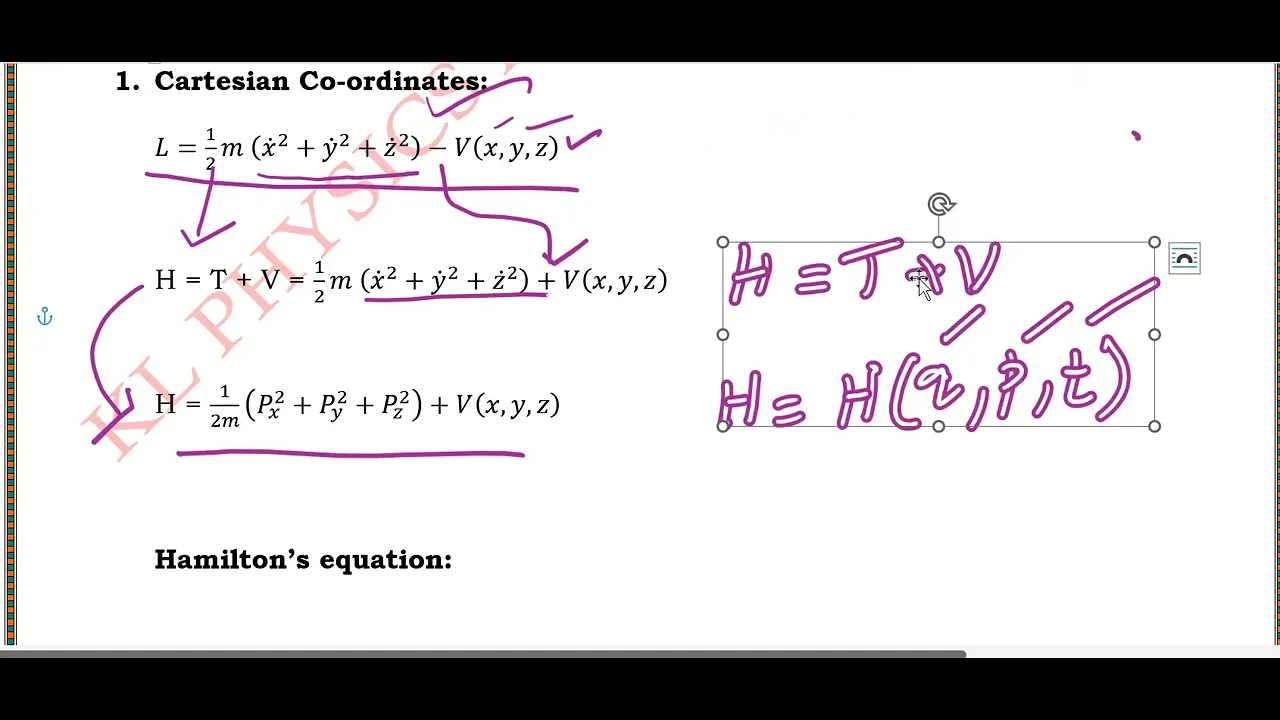
With Lrange, our starting point was the difference between the kinetic and potential energy. But with Hamilton, our starting point is their sum, which is the total energy or Hamiltonian. Now, for the simple pendulum we're working with here, the Hamiltonian is indeed the total energy. But this is not always the case. The more general definition of the Hamiltonian depends on the lrangeian and it's defined as this expression which might seem very confusing at first sight but I assure you it can be understood intuitively. We'll now take a useful detour to unpack this expression and understand the true relationship between the lrangeian and the Hamiltonian. The key idea here is a technical math term called the Leandre transformation, which is a way of transforming certain functions into new functions while still preserving all the information contained in the original. You might already be familiar with another way of doing this.
If you've ever encountered the Forier transform, for a given function f, you can apply the Forier transform to f and express f in terms of exponentials. The new function then is a sort of decomposed version of the original and contains all the same information. As a result, we have two different ways of encoding the same information.
The Leandre transform works in a very similar fashion. Suppose you have a simple single variable function called f. That is f only depends on the variable x. There are two ways that you can specify this function. The first is to say that for every value of x we assign a value f ofx. And by doing this for every point x we can specify the entire function.
But there is another way to do it.
Rather than assigning the value f ofx for a point x, we can instead assign the value of the slope of f at that point.
And we can similarly do this for every point x. So the tangent line to f or frime ofx is specified at every point x and by this method we can construct the whole function as long as we also specify the value of f ofx at some reference point say the y intercept.
This needs to be done because otherwise you can shift this graph up or down and if you only knew frime of x at every point then all of these would be equivalent. This is the essential idea behind what the leandre transformation is. In one instance, we have specified the information of the graph by assigning a value f ofx to each x. We can say that the pair fx encodes the information. Here in the other instance, we have used the slope at every point to specify the information. We'll call this new function based on the slopes s of x.
And since there's a onetoone correspondence between s and x, we can equivalently invert this function and consider a new function x of s. That is we are viewing x as a function of s.
Plugging this directly into f allows us to say that in this case we can consider f as a function of s. This brings us very close to the lejandra transform.
However, the true definition is that the Leandre transform of f is a new function g which is given by this expression. To understand why it has this form, we'll need to consider a more geometric approach. First, we draw the function f again.
We then select a specific value of x and draw a line connecting x to f ofx. The length of this line just equals the value of f ofx. So we'll call it f.
Next, we draw the tangent line to the curve at this point and note where it crosses the y ais. We call the length here g. So the y intercept is at y = g.
Now the slope of the tangent line is s.
We can therefore conclude that g + f = s * x. Slightly rearranging and recalling that we defined x as a function of s we arrive at the definition of the leandre transform. So the two ways we have of encoding the same information are given by these pairs fx and gs where g is the leandre transform of f. And since the leandre transform is its own inverse you can apply it again to g to arrive back at the original function f. We thus have a nice duality that encodes the information about our graph. The function f with independent variable x and the function g with independent variable s. The leandre transform is the tool that allows us to go back and forth between each of these perspectives.
So how does all this relate to the Hamiltonian? Well, remember how I said that for the simple pendulum, the Hamiltonian was just the total energy.
But the more general definition was this expression. Look at what happens if we apply a leandre transformation to the lrangeian. The lrangeian is a function of two variables q and q dot which are the generalized position and velocity respectively. Now, just as we were able to begin with a function f that depended on a single variable x and turn it into a new function g that depended on s, we can do something similar for a multivariable function. We just need to pick one variable at a time. In this case, since the lrangeian depends on q and q dot, we will keep q as it is. And our goal will be to transform to a new function that depends on Q and the derivative of L with respect to Q dot.
To do this, we just apply the formula we found for the Leandre transformation.
And we get that this new function equals the following.
Next, we define a new quantity that physicists refer to as the generalized momentum. Plugging it in gives this expression.
Finally, this is for just one degree of freedom. If our system had more degrees of freedom, we would need to sum over all of them. And now we can see that the Leandre transformation of the lrangeian is exactly the Hamiltonian.
Isn't that amazing? Just as the pairs f(x) and gs both encoded the information about the graph we considered, the lrangeian and the Hamiltonian do the same thing for the physics of a system.
Whatever information is contained in the lrangeian of a system is necessarily contained in the Hamiltonian as well.
It's just that the lrangeian encodes the information based on the generalized position and velocity. But the Hamiltonian encodes it based on the generalized position and momentum. Now you might be thinking okay great but what's the big deal? Momentum is really just P= MV right? It turns out, no, it's not. There are countless examples in physics where the notion of momentum equaling mass times velocity simply doesn't apply. To give you just one example, consider the motion of a particle that is moving near the speed of light. Since it's moving so quickly, we require special relativity to describe its motion.
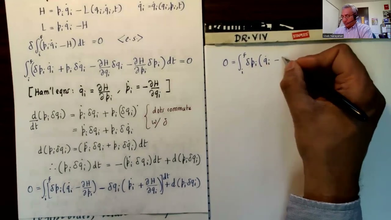
In this case, the lronian of the system is the following. And the momentum of the particle is not its mass times its velocity rather its momentum is given by the generalized momentum equation resulting in this expression which encodes Einstein's corrections to Newton. So the Hamiltonian truly gives us a totally different way to encode the same information that's contained in the lrangeian. And just as we use the lrangeian to write down the oiler lrange equations here we will use the Hamiltonian to write down Hamilton's equations for the simple pendulum. You'll recall that we had this Hamiltonian. Hamilton's equations are two equations of the following form. It's important to note here that while using the lrangeian approach we arrived at one second order differential equation. But with Hamilton's approach, we get two first order differential equations. They both lead to the same equations of motion. So it really depends on the specific problem you're tackling whether or not one approach has an advantage over the other. For example, if you are interested in numerically solving something, then you'll likely prefer the Hamiltonian approach as it's generally much easier to numerically integrate first order differential equations as opposed to second order ones. Okay, let's now see what we get if we carry out the calculations. First, we rewrite H in terms of P. Then the derivative of H with respect to P is just P / M R 2.
And the derivative of H with respect to theta is MGR sin theta, which means P dot is just minus this. So from Hamilton's equations, we get these two results. The top equation implies that P = theta dom.
We can take its derivative with respect to time and set it equal to the bottom term. Anceling like terms and rearranging, we get that theta dot equals g sin theta. The same exact equation we got with Lrange's approach. So whether we use the lrangeian or the Hamiltonian as our starting point, we arrive at the same equations of motion. Both approaches describe the same physics from two complimentary views. Moreover, since Hamilton's equations contained two first order differential equations, a new geometric view of the pendulum's motion opens up. We can see this by plotting the motion as a trajectory in something called phase space. We form a two-dimensional plot here where one axis is the position and the other axis is the momentum. Each of these lines here are curves or flows on phase space and they represent states of constant energy. So for any given curve, if you calculate the Hamiltonian of some point on it, you will always get the same result no matter which point you select.
We can then represent different states of the pendulum by points in this phase space. For example, if we start with one initial angle, it will follow this curve.
If we increase the angle, it will follow this one and so on.
Eventually, the motion becomes quite different if you release it with enough momentum. This type of geometric view has extremely general applications and can be used to shed light on all sorts of physical systems. For example, if we considered a simple harmonic oscillator, we can see that the motion is quite similar to the simple pendulum in phase space. What I'm actually showing here are 4,000 points with very tiny differences in initial conditions.
As you can see, they all evolve in exactly the same way.
If we inserted a damping force, then the motion begins to spiral toward the center.
This is because energy is not conserved here.
Eventually, the damped oscillator will come to a complete stop.
Finally, if we add a couple more terms, we get something called the duffing oscillator.
Plotting 4,000 points of slightly different initial conditions. Again, the phase space beautifully reveals the chaos in the system.
Now, everything I've mentioned is really just a teaser to the power of Lrangees and Hamilton's analytical approach to physics. These methods were further developed over the next century or so and have found their way into almost every area of modern physics. In fact, along with Carl Jacobe, Hamilton further refined his formulation of mechanics to arrive at something called the Hamilton Jacobe equation, which provided a sort of wave particle duality way of representing the motion of a particle.
It was this equation that heavily inspired a young Austrian physicist and led to his discovery of a new equation that would change the way we think about physics forever.
If you're interested in exploring some more fascinating math and physics topics, a great place to visit is this video sponsor, brilliant.org.
Their course catalog covers topics as diverse as calculus, circuits, number theory, and even how search engines work. Moreover, every single lesson will provide you with a fun, intuitive, and visual way to grapple with your understanding of any topic. You don't need to go it alone by banging your head against the textbook anymore. With Brilliant, you'll get instant feedback and know exactly where the gaps in your understanding are. Don't just take my word for it. Go check it out yourself.
You can begin learning for free on Brilliant right now by either going to brilliant.org/abidebyreason, scanning the QR code on screen, or clicking on the link in the description.
They've also given my viewers 20% off an annual premium subscription, which gives you unlimited daily access to everything on Brilliant.
Up Next
106:33
Quantum Mechanics Introduction: States, Vectors & Lecture 1
@stanford
910.9K views•2012-02-17

12:53
21cm Hyperfine Transition in Neutral Hydrogen: Radio Astronomy Basics
@AaronRobertParsons
12.4K views•2011-10-13

32:32
NMR Spin Physics I: Zeeman Effect, Resonance Condition & Larmor Frequency
@nptel-indianinstituteofsci8064
2.3K views•2024-01-17

27:14
Entropy and the Second Law of Thermodynamics Explained
@veritasium
27.5M views•2023-07-01
Related Study Plans & Knowledge Roadmaps
Structured learning paths in Physics
physics
Nuclear Physics (Decay, Fission & Reactors)
01Atomic Structure and the Binding Force
02Radioactive Decay and Half-Life
03Nuclear Fission Mechanics and Chain Reactions
+ 2 more learning modules
12h5 modules
Explore Roadmap
physics
Soft Matter (Polymers, Colloids & Rheology)
01Foundations of Soft Matter & Thermal Forces
02Polymer Physics and Macromolecules
03Colloids, Surfactants, and Self-Assembly
+ 2 more learning modules
38h5 modules
Explore Roadmap
physics
Analytical Mechanics: Lagrangian & Hamiltonian
01Mathematical Foundations: Calculus of Variations
02From Newtonian Mechanics to Constraint Dynamics
03The Principle of Least Action & Lagrangian Mechanics
+ 3 more learning modules
28h6 modules
Explore Roadmap
physics
General Relativity (Spacetime & Cosmology)
01Foundations of Relativity: Special Relativity
02The Geometry of Spacetime: Equivalence Principle & Curvature
03Einstein's Field Equations: The Mathematics of Gravity
+ 2 more learning modules
55h5 modules
Explore Roadmap