




















In classical mechanics, generalized coordinates are independent parameters that describe a mechanical system after accounting for constraints, reducing the number of degrees of freedom from 3N for N particles to 3N-K when K holonomic constraints are applied; these coordinates enable the Lagrangian formalism by providing a minimal set of variables that fully specify the system's configuration while respecting all constraints.
Classical Mechanics: Generalized Coordinates | Lecture 2
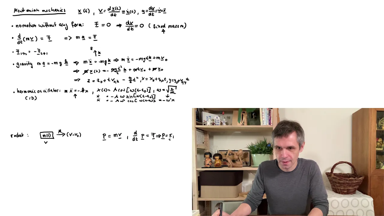
Added:Newtonian mechanics, including Newton's laws of motion, force vectors, and equations of motion in Cartesian coordinates.
Basic multivariable calculus, specifically partial derivatives, the chain rule, and total differentials.
Fundamental definitions of kinetic energy, potential energy, and angular momentum for point particles.
The concept of degrees of freedom in physical systems.
Formulating and solving the Euler-Lagrange equations to find equations of motion for complex systems.
Hamilton's Principle (the Principle of Least Action) as the variational foundation of Lagrangian mechanics.
Identifying cyclic coordinates and applying Noether's Theorem to find conserved quantities (integrals of motion).
Transitioning to Hamiltonian mechanics by defining generalized momenta and constructing the Hamiltonian function.
Analyzing constraints in multi-body systems, such as rigid body dynamics or the double pendulum.
71.7K views627likes45:49Original Release: 2012-12-17
so uh let me just make a few corrections to what I said in the previous lecture it was a student up here and uh showed me that I've been a little bit sloppy in writing a few of the equations so uh one thing that I did was that I [Applause] wrote I think I wrote this where we discussed the the equation describing the time derivative of the angular momentum so somewhere along the derivation I wrote this this should be fji and when I was discussing Central no conservative systems I wrote that for conservative systems the force can be written in this way mathematically due to this property that the closed loop integral from point from one point to the same point has to be zero uh what I should have done here is just to add a vector sign above the r because in general the potential can have a directional dependence on the position Vector so if there's no Vector here it means that the potential only has a radial dependence which is the same as a central Force so that it's just a detail so to be completely General I should have add a vector sign about the r and I also received a question about the exercises in this course the written exercises and they are not mandatory so you don't have to hand them in however I strongly recommend that to do them if you want to get a good grade at your exam and learn the physics in this course you have to do the the exercises no doubt about it okay so we were discussing uh the content of the angular momentum of the system what does it consist of and uh we had introduced these various vectors we had introduced the reference system with the orgo the center of mass and the position Vector to some particle I and then we introduce these relative vectors primed vectors which essentially are the difference between the position Vector to particle I and the center of mass position [Applause] vector and the reason why we do this will now become uh clear we start out again with the general definition of the total angle momentum in the system just the sum over all the angular momenta of each particle I and using these definitions I can rewrite this equation like this so I get four terms m [Applause] if I just multiplicate out all of these terms in this equation I get four terms like this so now the task is to try to attach some physical meaning to each of these terms what do they represent physically what well before doing so there's at least one simplification we can actually do and that simplification is to set these terms equal to zero so please take one minute to discuss with your neighbor why are these terms equal to zero all right any ideas why are these terms equal to zero no ideas so not that the relative Vector here r i Prime can write this as so it's the difference between the position Vector RI and the center of mass coordinates large R and we also have a sum over I involved well the reason is that we have actually a cancellation of terms and we can see this by using the definition of the cent of mass coordinates so these two terms are actually Zero by definition so we have and then recall the definition of the the center of mass coordinate so let's insert this into the equation so we get this now this term is independent on I so the only summation of I regarding this last term is related to Mi this is just a total mass of the particles in the system so this term cancels comes one so we end up with this which is zero because I can call I can rename the synthesis to I if I like so that's pretty significant simplification of this equation these two terms cancel so we're left with these terms for and we get this large M because the only term here which is depending on I is MI so the sum of I just becomes large M and now perhaps we can say something about the physical meaning of the content of the angular momentum this first term involves only quantities related to the center of mass contains Center of mass position the total mass of the system and the velocity of the center of mass so this first term can be interpreted as the angular momentum relative the origo of the coordinate system as if all the mass of the system was located in the Central Mass so this is the center of mass term now what about the second term well we see that it only involves relative vectors it involves the relative position of particle I relative the center of mass and the momentum of particle I relative the Central Mass so the last term actually describes the angular momentum relative the center of mass okay so let's try to VIs visualize this physically let's say my hand here is the Oro of the cordinate system this is the system with all the particles if this is moving in some kind of orbit without changing its position relative its Center of mass only the first term is non zero right because there's no relative motion of the particles in the system relative to center of mass just moves like a hole but if there is motion relative my hand however if I now take this compendium and see if I can do this if I spin it while it rotates then I have two kinds of rotation I have one rotation relative the orgo but I also have an internal rotation relative the center of mass so can of spins uh simultaneously as it rotates so that's the second term because it only consists of the relative position and relative momentum uh so you could we could rephrase this as the internal spin of the system which we can say so yet another scenario is that if the center of mass is not moving relative to orgo but only spins around itself then only the last term is non zero whereas the first term is zero do you have any questions related to this okay so we see that the total angular momental of system can be divid into two parts the internal Spin and sort of the angular momentum of the system as a whole represented by the centeral mass now the question is can we do something similar for the kinetic energy of a system well it turns out that we can actually split the total kinetic energy of the system again into one Center of mass part and one uh sort of internal part so again I use this definition of the relative velocity Vector so what really interest here uh are the velocities of particle I VI and VI but I rewrite this in terms of the Central Mass velocity and the relative velocity of particle I with respect to the center of mass just as we did for the angle momentum and if I just do the multiplication here I get I get the following so I also get four terms but two of them are the same and combine into this term as we saw just 5 minutes ago this this last term is zero by definition so the kinetic energy can be Rewritten as a center of mass term the the velocity of the cent of mass as if all the mass was gathering into one point and moving in addition to the relative velocities of the particles with regard to the center of mass so then I have one question let's say that we're dealing with a rigid object uh this desk is rigid enough for our purposes it means that it's solid I can't deform it not easily anyway so this point will always be fixed compared to this point for instance it's rigid does this mean that the second term is zero no why not you rot right so just to repeat for the uh recording if you rotate the particles they will still move so we're not only this term not only describes a physical deformation of the object but it also describes uh a relative rotation of the particles compared to the Central Mass so similarly you can actually have an object which is standing still but if it's rotating it still has kinetic energy and that is precisely what is described by this term so this is the center Master this is the internal kinetic energy for instance describing rotation okay we'll now try to say something about a concept which is often used in realistic systems namely constraints if we were to describe for instance a system of a gas a system of particles trapped in some container we would have to use some constraints namely the fact that the particles cannot move outside the container right so there's some kind of boundary condition at the walls which prohibits the particles from escaping so how do we take into account constraints when describing and wanting to solve various mechanical problems so one example is a gas with particles uh in some container another example is some ball rolling down a hill and I use these two specific examples because I want to introduce a type of classification for constraints because you can have you can have different types of constraints one type of constraint is known as a holonomic constraint and a holonomic constraint can be written the following way uh it's a function of the particles R1 R2 Etc and all the particles in the system and possibly even time and it has to be equal to zero an example of such a constraint is a rigid body because the equation describing some rigid body can can actually be written quite generally like this so This expresses that the relative position Vector the magnitude since we Square here the the magnitude of the relative position between two points in the rigid body has to be the same it means that you can't deform the body you can still have a rotating body you just can't deform it you can't change distance between the particles this has precisely the form of a holonomic constraint which can be made obvious by writing the equation like this well if you have holonomic constraints you might have guessed that there's also possible it's also possible to have nonholonomic con constraints and non Hol number constraints cannot be written like this so if you consider this ball rolling down the hill uh this is actually an example of nonholonomic constraint to make it a little easier let's assume this hill incidentally has the form of a perfect circle with some radius a so then the physically allowed space where the ball can move is everywhere here except inside uh the hill so basically if R describes the position Vector to the ball then R 2 - A squ has to be greater than Z if it's zero it's moving along the hill but if it's jumping for instance bouncing then it's greater than zero so basically this is a nonholonomic constraint because you don't have an equality sign here you have an inequality sign so let me Al also just mention briefly two types of classifications which are related to the time dependence of the constraints you have something known as romic constraints which are time dependent constraints and you have scaron constraints which are time independent so these are a lot of words um what we'll be dealing with mostly are holonomic constraints but it's good for you to be aware of these very specifications so this was basically so far uh well up to constraints mainly a repetition of stuff which I think most of you have seen in some form or another previously uh and now we're actually moving towards actually our first encounter with this earlier mentioned lran formalism which will prove to be a very useful tool for us to and it sort of gives us a a general prescription for how to address problems in mechanics mechanics as a general procedure for how to solve them and related to this lran formalism is an important concept known as generalized coordinates so again we confine our discussion to a system of many particles assume we have large n particles if you allow all of these particles to move in three dimensions we will have three n number of independent coordinates but let's say we want to incorporate now constraints to the system we assume that there are some kinds of constraints which are valid for our system and let's say we have a number of K constraints and we assume these are holonomic for Simplicity so we assume there are a number of K constraints which can be written like this so it means that if we have originally 3 m independent coordinates with k constraints we have 3 m minus K independent coordinates in reality when take into account these constraints and we denote this new set of independent coordinates as Qi so that if r i are the original 3 n degrees of freedom then Qi are these new independent degrees of freedom when taking into account these K constraints so let me write this so we start with a description of the system uh where each particle is described by r i so we have r one describes particle one R2 describes particle 2 Etc up to particle m sorry so when we take into account the constraints it means that all of these original degrees of freedom are no longer independent they can be described in terms of these new generalized coordinates Qi we see that we have 3 n minus K degrees Freedom which are independent so it means that not all of these r i R1 R2 up to RN can be independent you see what I mean so these The Q's are now the independent coordinates where the constraints have been taken into account whereas the RS are the original it's the original description of the system without taking into account the constraints so you can think of these this set of equations as a set of transformation equations taken from from the original description to these uh new generalized coordinates or vice versa by including the constraints in the system so this might seem a bit abstract so let's consider a concrete example so what we have here uh is for instance a ceiling and we have a double pendulum so we have one spherical uh ball for instance hanging from the ceiling by some uh rope and attached to this one is a second bow with another rope here and let's assume this rope is in fact uh a bar which is rigid so you can't deform it now in principle if this system can move in three dimensions we would have how many degrees of freedom would we have two particles six three for each particle let's confine the discussion to a plane so these particles are now only allowed to move in a plane how many degrees of freom do we have them four why exactly so in principle for this system we should have four degrees of freedom however as we fix the distance here by saying that this ball is connected to the ceiling by a bar which cannot be deformed we're removing one degree of Freedom we we are removing one degree of freedom for each ball so DF degrees of freedom is a we have two so we're doing this by saying that distance between these points and these point and these two points uh are fixed so the only degrees of freedom we have in the system are in fact the angles here Theta 1 and Theta 2 which are describing how these objects are moving relative each other so the generalized coordinates for our system here are Theta 1 and Theta 2 let's try to see how this relates to this set of transformation equations let's say that origo for our reference system is located here so if the position of particle one just wanted to make it a right hand system uh okay so X is going down Y is in this direction so we see then that the X position of particle one should then be R1 cosine th 1 y1 should be R1 sin Theta 1 these are just polar coordinates but in fact this is just L1 or cosine th 1 and L1 sin th 1 so if we were to write this transformation equation for our system we should have you see that it's only a function of theta one right in principle it could have been a function of theta 2 as well but it's only a function of the generalized independent coordinates of the system these two coordinates are independent all the other coordinates are depending on each other so do you see the difference between the original set of coordinates which are used to describe the system and the set of independent generalized coordinates when you take into account constraints in the system okay I see some nodding heads right all right having introduced these uh the notion of generalized coordinates we're actually ready to take the step onto deriving the lrange equations which would be the most which would be the equations you use most in this course oh that was beautiful equation in addition to these generalized coordinates we have to introduce a concept known as a virtual displacement so I'll just Define it here so a virtual displacement is defined as an infinitesimal displacement of the coordinates of the system which are in accordance or Allowed by any possible constraints that may be possible in the system so if we revert to our example of the ball rolling on a hill an allowed virtual displacement would be up or along the hill but not into the hill that would be in um that would not be allowed in terms of the constraints of the system [Applause] assume first that we have a system which is in in equilibrium and by that I mean that the net force acting on each particle is zero and if each force is zero then it's trivial to see that the sum of each Force dotted with this virtual displacement Vector also has to be zero because each term is zero and let me now assume that this total Force fi this can be split into two parts so I've split the total Force AC particle I into an applied force and a force coming from the constraints of the system so for instance a gas with particles inside a container in this context the constrainted force would be the force acting on the particles by the wall when they're bouncing against the wall whereas an applied force would be if we change the pressure in some way for instance so this part of the force stems from the constraints and this is an applied force from us The Observer for instance y yes okay I think uh we'll call it there so remember the guidance hour is on Friday from 2 to three
Up Next
18:22
Euler-Lagrange Equation Explained Intuitively | Lagrangian Mechanics
@EugeneKhutoryansky
444.8K views•2018-11-18

12:53
21cm Hyperfine Transition in Neutral Hydrogen: Radio Astronomy Basics
@AaronRobertParsons
12.4K views•2011-10-13

32:32
NMR Spin Physics I: Zeeman Effect, Resonance Condition & Larmor Frequency
@nptel-indianinstituteofsci8064
2.3K views•2024-01-17

27:14
Entropy and the Second Law of Thermodynamics Explained
@veritasium
27.5M views•2023-07-01
Related Study Plans & Knowledge Roadmaps
Structured learning paths in Physics
physics
Nuclear Physics (Decay, Fission & Reactors)
01Atomic Structure and the Binding Force
02Radioactive Decay and Half-Life
03Nuclear Fission Mechanics and Chain Reactions
+ 2 more learning modules
12h5 modules
Explore Roadmap
physics
Soft Matter (Polymers, Colloids & Rheology)
01Foundations of Soft Matter & Thermal Forces
02Polymer Physics and Macromolecules
03Colloids, Surfactants, and Self-Assembly
+ 2 more learning modules
38h5 modules
Explore Roadmap
physics
Analytical Mechanics: Lagrangian & Hamiltonian
01Mathematical Foundations: Calculus of Variations
02From Newtonian Mechanics to Constraint Dynamics
03The Principle of Least Action & Lagrangian Mechanics
+ 3 more learning modules
28h6 modules
Explore Roadmap
physics
General Relativity (Spacetime & Cosmology)
01Foundations of Relativity: Special Relativity
02The Geometry of Spacetime: Equivalence Principle & Curvature
03Einstein's Field Equations: The Mathematics of Gravity
+ 2 more learning modules
55h5 modules
Explore Roadmap