















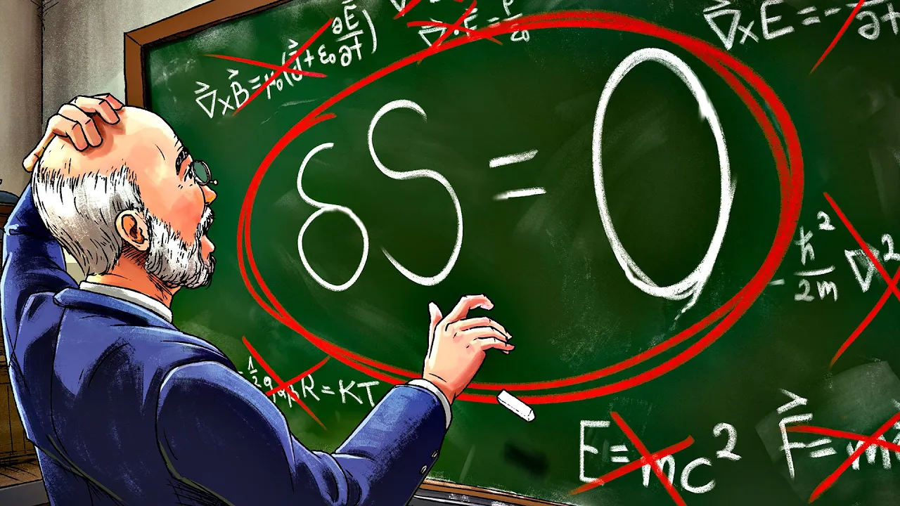
![МИ НАБЛИЗИЛИСЬ ДО ТЕОРІЇ ВСЬОГО [VERITASIUM]](https://i.ytimg.com/vi/FhQXcvnR-0U/maxresdefault.jpg)

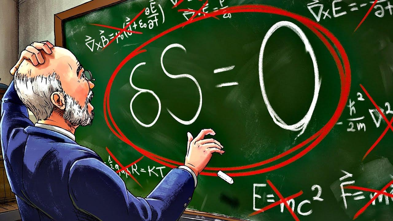








Lagrange's method provides a systematic approach to deriving equations of motion for mechanical systems by using generalized coordinates (which don't need to be Cartesian) and applying the Lagrangian equation: d/dt(∂L/∂q̇_j) - ∂L/∂q_j = Q_j, where L = T - V (kinetic minus potential energy), and Q_j represents generalized forces from non-conservative forces. The method requires choosing independent, complete, and holonomic coordinates (where degrees of freedom equal the number of coordinates needed), then computing four terms for each coordinate: the time derivative of the partial derivative of kinetic energy with respect to velocity, minus the partial derivative of kinetic energy with respect to position, plus the partial derivative of potential energy with respect to position, equaling the generalized force obtained through virtual work calculations.
Lagrange's Method with Examples | MIT 2.003 Engineering Dynamics
Added:The following content is provided under a Creative Common License. Your support will help MIT Open Courseware continue to offer highquality educational resources for free. To make a donation or to view additional materials from hundreds of MIT courses, visit MIT Open Courseware at ocw.mmit.edu.
All right, let's get started. Today's all about Lrange will method. We will talk a lot about what we really mean by generalized coordinates and generalized forces and then do a number of application examples.
There's a set of notes on stellar on the Lrange method. It's about 10 pages long and I highly recommend you you read them. They're they're they're not somehow up with the notes associated with lecture notes. They're kind of in a way down at the bottom. So, you have to scroll all the way down in the stellar website to find them.
The uh there's our second quiz is November 8th. That's a week from next Tuesday. Okay. Pretty much same format as the first one. Okay.
So let's talk about how to use lrange equations.
So I defined what's called the lrangeian last time.
T minus v the kinetic energy minus the potential energy of the entire system.
Total kinetic and total potential energy expressions.
Then we have some quantities QJs.
These are defined as the generalized forces generalized discoordinates I should say and the capital Q subjs are the generalized forces.
Okay.
And the lrangege equation says that d by dt the time derivative of the partial of l with respect to the q j dots the velocities minus the partial minus the partial derivative of L with respect to the generalized displacements equals the generalized forces. And in for a typical system, you'll have a number of degrees of freedom like say three. And if you have three degrees of freedom, you need three equations of motion. And so that you're the J's will go from one to three in that case. So the J's here refer to an indicy that gives you the number of equations that you need. So you do this calculation for coordinate one again for coordinate two again for coordinate three and you get then three equations of motion. Okay. So this is a little a little obscure. I like to let's just plug in for L= T minus V and just put it in here and see what happens.
You get d by dt of the partial of t with respect to q j dot minus d by dt of the partial of v with respect to q j dot plus I'll organize it this way minus the partial of T with respect to Q J plus the partial of V with respect to QJ equals capital QJ.
Now when we first talked about potential energy a few days ago, we said that for mechanical systems the potential energy is not a function of time or anybody remember velocity.
So if the potential energy is not a function of time velocity, what will happen to this term?
Goes this goes away. So this is zero for mechanical systems.
You know, if you start getting into electrons moving in magnetic fields, then you start having potential energies involving velocities. But for mechanical systems, this term's zero. And I think the bookkeeping though, so this is the form of lrange equations that I write down when I'm doing problems. I don't write this. Mathematicians like you know elegance and this comes down to this beautifully elegant simple looking formula but I'm an engineer and I like it to be efficient you know and and practically useful. This is the practically useful form of lrange equations. So you just use what you need potent kinetic energy here kinetic energy there potential energy there. And I number these.
There's a lot of bookkeeping in Lrange.
So I call it term one, term two, term three, and term four because you have to grind through this quite a few times.
And so when you do, basically, you take one the results of 1 + 2 + 3 = 4. And you do that uh j times to get the equations you're after.
Okay.
So a little now we need to talk a little bit about what we mean by generalized coordinates.
QJ general. What you know what's this word generalized mean? Generalized just means it doesn't have to be cartisian.
Not necessarily cartisian as in xyz.
You have a lot of liberty in how you choose coordinates. Not necessarily cartisian. Uh not even um inertial.
They do have to satisfy certain requirements. The coordinates they must be what we call independent.
They must be complete and so they must be independent and complete and the system must be holic.
Now I'll get to that in a minute. So we need to you need to understand what it means to be independent, complete and whole and so what do we mean by independent?
So if you have a multiple degree of freedom system and you fix all but one of the coordinates, you say system can't move in in all but one of its coordinates, that last degree of freedom still has to have a complete range of motion. So if you have a double pendulum and you grab the first mass, the second mass can still move. It takes two angles to define your double pendulum.
So independent when you fix all but one coordinate.
still have a continuous range of movement in essentially in the free coordinate.
And that's independence.
And we'll just we'll just kind of use the we'll we'll uh do this by example mostly. and complete the to complete really means it's capable of locating all parts of the system at all times.
Okay.
So let's think about let's look at the system here. It's double pendulum.
It's a simple one just made out of two particles.
and strings. I should have didn't bring one today.
And I could I need to pick some coordinates to describe this.
Okay. And we'll put this in a uh we'll use some cartisian coordinates here. Say an x and a y. And here's particle one.
And I could choose to describe this system co uh xy coordinates. And I'll specify the location of the system with coordinates x1 and y1. Two values to specify the location of that. And I'm down here. I'm going to pick two more values x2 and y2 to describe the uh so these are the x1 is a different coordinate from x2. x1 is the x position of particle one. x2 is the x position of particle 2. Y1 and y2.
Okay.
So, how many coordinates do I have to describe this system?
How many have I used?
Four. Right. How many degrees of freedom do you think this problem has?
Two. Right. So, there's something already a little out of whack here. Um, okay.
But the point is these aren't independent. You'll find you just do a test, you find that these aren't independent. If I fix x1 and x2 systems doesn't move right.
I say this has got to be one and this has got to be three. It this system is now frozen.
So this system of core coordinates is not independent.
What do we say independent? When you fix all but one coordinate, you still have continuous range of movement of the final one. I can fix only just two of these and I've frozen the system. I don't even have to go to the extent of fixing three.
I'm assuming the strings are of fixed length. You can't change the string length. Okay. So, this is not a very good choice of coordinates. And we had a hint that it might not be because it's more than we ought to use. We only really need two. Okay. Okay. So, and then if we choose these angles F1 and F2, let's do the test with that. Are those independent? So, if those are the coordinates of the system, if you fix F1, is there still free and continuous movement of F2 of the system? Sure. And if you fix V2, which means you can require this angle stay rigid like that and move F1, well, the whole system will still move. So Fe1 and Fe2 are a system which satisfies the independence requirement complete. They're both systems are complete. They're both capable of locating all points at all times.
Okay? But only the pair f1 and f2 in this example are both independent and complete.
Now the third requirement is this thing thing called hol holomicity.
And what holen what it means to be holomic is that the system the number of degrees of freedom required is equal to the number of number of coordinates required to completely describe the motion. Now, most of the time, every example we've ever done so far in this class satisfies that. We pick V1 and V2, and that's all the coordinates we need to completely describe the motion. Let me see if I can figure out a uh a counter example.
So, I did I I didn't write down this definition. So, holomic And if the answer to this question is no, you cannot use lrange equations.
So let's see if I can show you an example of a system in which You need more coordinates than you have degrees of freedom. I've got a ball.
It's on the X. This is an XY plane.
And the I'm not going to allow it to translate in Z.
And I'm not going to allow it to rotate about the Z-axis.
So I'm constru.
So this is one rigid body. How how many general how many degrees of freedom does it have?
Six. Okay. I'm going to constrain it. So no Z motion. Five. No Z rotation. Four.
I'm not it's is not going to allow it to slip. This is X and that's Y. I'm not going to allow it to slip in the X.
So now I've got another that's one. Now I'm down to three. And I'm not going to allow it to slip in the y two. So that by our calculus of how many degrees of freedom you need, we're down to two. We should be able to describe completely describe the motion of this system with two coordinates. Okay. So I've got this put this piece of tape on the top and it's pointing diagonally that way. And I'm going to roll this ball like this.
until it shows up again. So, it's right on top just the way it started.
Okay. Now, start off the same way again.
I'm going to roll first this way and then I'm going to roll this way to the same place.
Where's the stripe?
It's in the back.
So, I've gone to the same position, but I've ended up with the ball not in the same orientation as it was. I went by two different paths and the ball comes out over here rather than up there where it started. Okay. So this system actually to actually describe where the ball is at any place out here having gotten there by running around rolling around without slipping and without Z rotation.
How many coordinates do you think it'll take to actually specify where that stripe is arbit at any arbitrary place that it's gotten to on the plane?
Name them.
distance rotation.
So you got in order to actually fully describe it, you got to say where it is x and y and you actually have to say some kind of theta and fe rotations that it's gone through so that you know where this is. Okay. So this system is not holomic and holomic. It has to be holomic in order to be in order to use lrron's equations.
Okay, so when you go to do Lrange problems, you need to test for your coordinates complete, independent, and holomic. And you get pretty good at it. So So here's my lrangee equations and I've itemize these four calcula calc calculations you have to do column 1 2 3 and four. Okay. And so what I just want what I want to write out is just to show you just to get you to adapt a systematic approach to doing lrange. So, left hand side. So, the left hand side of your equations of motion is everything with T and V. The right hand side is has these generalized forces that you have to deal with. And the generalized forces are the non-conservative forces in the system.
Okay. So, this is going to get a little bit cookbook, but it's I think you appropriate for the moment here. So step one, determine the number of degrees of freedom that you need and choose your delta J's. Those are your not deltas, excuse me, just qjs.
Choose your coordinates. You find the number of degrees of freedom and choose the coordinates you're going to use.
Basically verify complete independent Polomic three.
Compute T and V for every rigid body in the system. Compute your kinetic and potential energies.
One, two, three for each qj. So for every coordinate you have, you have to go through these computations. 1 2 3 4 for every coordinate.
And this is your left hand side.
And if you don't have any external forces, any non-conservative external forces, then 1 2 1 plus 2 plus 3 equals zero. But if you have non-conservative forces, then you have to compute the right hand side. So the right hand side.
So for each qj each generalized coordinate you need to find the generalized force that essentially goes with it.
And you do this by computing the virtual work delta W. I'll put the little NC up here to remind you these are for the non-conservative forces. The delta W associated with the virtual displacement delta qj. So for every generalized coordinate you have, you're going to try out this little delta c delta of motion in that coordinate and figure out how much um virtual work you've done. So so delta wj is going to be qj delta j. So whatever this is the thing you're looking for.
And it's going to be a function of all those external non-conservative forces acting through a little virtual displacement. A little bit of work will be done. Mostly I'm going to teach you how to do this by by example.
[Music] So let's quickly do a really simple trivial system.
Our mass spring dash pot system single degree of freedom m k b it's going to take one coordinate to describe the motion.
X happens to be cartisian.
There'll be one generalized coordinate.
So Q J = Q1 equals QX in this case. It's our X coordinate. Actually I should just call it X. That's our generalized coordinate for this problem. Is it complete? Yep.
Is it independent? Yes. Is it whole? No problem. Okay, we need t m x dot squared. We need v and we have 12 k x^2 for the spring minus mgx for the gravitational potential energy.
And now we can start and we have some external non-conservative forces. What are they fi non-conservative?
And I think I'll better I'm going to put an excitation on here too. Some f of t.
So what are the non-conservative forces Jonathan? Pardon?
K. It's not K, but oh, I wrote my mistake. Sorry about you're correct. I'm just uh my brain is getting ahead of my writing here. That's normally B and this would be K. I'm not trying to really mess you up there. So, what would that it would be Bx dot, right? Okay. Right. And is there anything else?
Are there any other non-conservative forces? Things that can put energy into or out of the system?
So the damper can certainly extract energy.
F.
Yeah, the forcef that external it might be, you know, something that's making it vibrate or whatever, but it's an external force and it could do work on the system and it's not necessarily a it's not a potential. It's not a spring and it's not a it's not gravity.
It's coming up and somebody's shaking it or something like that. So F is also non-conservative. So the non-conservative forces in this thing are uh F in the I direction and minus Bx dot in the I direction. And we could in our normal approach using Newton, we'd draw a free body diagram and we we'd identify a BX dot on it and an F on it, but we'd also have our kx on it.
That would be what our free body diagram would look like. And the non that's a conservative force. Oops. And we need an mg.
So we have two conservative forces kx and mg. And we have two non-conservative forces bx dot and f. So in this case the non-con sum of the non-conservative forces is f in the i direction minus bx in the i x dot in the i direction.
So let's do our calculus here. So 1 d by dt of the partial of t which is 12 m x dot squared with respect to x dot.
So that gives me the derivative of x dot^2 with respect to x dot gives me a 2 mx dot. So this is d by dt of mx dot but that's m x dot. And as you might expect when you're trying to drive equation of motion you're probably going to end up with an mx dot in the result and it always comes out of these dydt expressions.
Okay. So that's term one.
term two in this problem minus t with respect to x in this case is t a function of x say 12 mx dot squared but so is t a function of displacement x it's a function of velocity in the x direction but is it a function of displacement no so this term is zero three our third term partial of v with respect to x ah well where's v half kx^2 the derivative of this is kx minus mg okay and we sum those So we get mx dot plus kx - mg equals and on the right hand side this is four.
Now we need to do four for the right hand side and four is really the summation of the FIS the individual forces dotted with dr. These are both vectors.
dr is the movement. little bit of work and it's going to be a delta quantity like delta x and f of the applied forces and you need to sum these up. So this dr in general is going to be a function of the delta j's the virtual displacements in all the possible degrees of freedom of the system. We do them one at a time. This case we only have one so it's trivial but this could be you know delta 1 2 3 4 and each one of them might do some work when f moves through it but work is f dot the displacement so it's the component of the force in the direction of the movement the dotproduct that gives you this little bit of virtual work okay so in this problem this is going to be equal two, we actually have an f of t some function of time in the i direction minus b x dot in the i direction dotted with delta x which is our virtual displacement in our single generalized coordinate. And this whole thing is going to be equal to q x delta x.
So you figure out the virtual work that's done.
So delta. So if you do this dotproduct, this is also in the ihat direction. into I do I I do I you just get ones because the forces are in the same direction as the dis as the displacement you're going to get an FT f of t delta x is one of the little bits of virtual work and you'll get a minus bx dot delta x and that together those two pieces added together are the generalized force times delta x This total here gives you delta w non-conservative for in this case coordinate x.
So we need to we're trying to solve for the what goes on the right hand side. We need the qx.
So we have here you notice what'll happen. you'll divide, it'll cancel out the delta x's that result.
And in this case, what you're left with is qx = f of t minus bx dot.
So this is number four.
So qx delta x is the bit of virtual work that's done what goes into our equation of motion is the qx part and we got it by computing the virtual work done by the applied external non-conservative forces as we imagine them going through delta x and we're done. And you have the complete equation of motion for a single degree of freedom system. You could rearrange it a little bit. mx dot plus bx dot plus kx equals mg plus f of t if you will. So it's the same thing you would have gotten from saying from using Newton in a you know in a trivial kind of example but it helps define each of the steps things that we said were required.
Okay. So, we're going to go from there to a much harder problem.
So, any issues or questions about definitions, procedure?
So, when you start getting into multiple degrees of freedom, you need to set up a careful bookkeeping.
So, I I do I just do this myself. Then I I top of the page, I identify my coordinates.
I write down t, write down v. Then I say, okay, coordinate one, one, two, three, four equation. Then I start with a coordinate two. Calculus for one, two, three, and four and so forth till you get to the end. Okay, questions. Yeah.
on the line.
Um, what's that thing?
Oh, I these are functions of the of the delta J's. this this DR where it comes from the work that's being done in the virtual displacement around a dynamic equilibri equilibrium position for the system is a little movement of the system Dr. and we express it it's expressed in terms of the generalized a virtual displacement of the generalized coordinates of the system. So where the dr comes from is going to be delta in this case it's only delta x and in the next problem we're going to do the force in the problem is not in exactly the same direction as the delta x's and delta thetas and so forth. So when you do the dotproduct only that component of the force that's in the direction of the virtual displacement does work and you you account for that.
So let's let's uh look into a more difficult problem.
So the problem is this. I tried to I I tried to fix this up before I came to class and I really didn't really quite have the the uh parts and pieces I needed, but this is a piece of just a piece of steel pipe here. It's a sleeve on the outside of this rod.
And I've got a spring that's on the outside connected to this piece. And so it can do this.
Okay. And it's also though a pendulum.
So the system I really want to look at is this system.
So as it swings back and forth, the thing slides up and down.
So this has multiple sources of kinetic energy, multiple forms of potential energy. Okay? And I'll for the purpose of the problem, I'm going to say that there's a force that's always horizontal acting on this mass pushing this system back and forth. Some F cosine omega t always horizontal. And I want to drive the equations of motion of the system.
So, is it a planer motion problem?
All right. How many rigid bodies involved?
Okay. So, you know, for so there's two there's two rigid bodies. Each could have possibly six degrees of freedom.
But when you say it's uh planer motion, you're actually immediately confining each rigid body to three. Each rigid body can move X and Y and rotate in Z.
So the number when you thread out now say this is planer motion you've just said each rigid body has max three. So this has a maximum of six possible right? No the other where the other three disappear too is no Z deflection and no rotation in the X or Y. Okay. So we have a possible uh possible maximum six. How many degrees of freedom does this problem have? How many coordinates will we need to completely describe the motion of the system? So, come up. So, think about that. Talk to a neighbor. Decide on the coordinates that we need to use for this system. And while I'm drawing it, Okay. What do you decide? How many?
Two. All right. What would you recommend?
What would you choose?
Pardon?
The angle.
an angle and a deflection of what I'm calling M2 here.
Okay, so this is M2, the rod is M1, and he's suggesting an angle theta, and a deflection, which I'll call X1. And I've attached to this bar, the rod, I'm calling it, a rotating coordinate system, x1 y1 about point a. So a x1 y1 is my rotating coordinate system attached to this rod.
Okay. So, I'm going to locate the position of this by some value x1 measured from point A and locate the position of the rod itself by an angle theta. Good.
Is it complete? So, if you freeze one, do you still have uh complete? Does it again? Can you describe the motion at any possible position?
Those two things. Yes. Is it independent?
If you freeze x, can theta still move?
If three is the can the x still move okay is it whole and right two equals you know you need two we got two and they're independent and complete good so now the harder work starts so I'm going to give us the mass of the rod the mass moment of inertia of the rod about the zaxis about with respect to a the length of the rod is l1 the sleeve mass m2 gi iz with respect to its G. So it has a G. They there's also I better call it G2.
That's the G of the sleeve. There's also a G1, a uh center of mass for the rod and a center of mass for the sleeve. We those are properties we'll need to know and I'll give them to you.
Okay.
So we need to come up with expressions for potential energy and kinetic energy. So this this problem the connect potential energy is a little messy because you have to pick references you have to account for the unstretched length of the spring.
Right? So uh call L0 is the unstretched spring length give it we know that also. So I propose that the potential energy look like 1/2 for the spring. Anyway, one half the amount that it stretches in a movement x1.
The amount that it stretches then should be whatever that x1 position is. And that x1 position and I have just I drew it slightly incorrectly. I'm going to use X1 to locate the center of mass, which is always a good practice. So, here's the center of mass. So, my X1 goes to the center of mass.
Okay, that's X1.
So, that the that's the total distance.
And from that we need to subtract L0 the unstretched length of the spring and we need to subtract half the length of the body because it's going that that's that extra bit here. Okay. So this is the amount that the string is actually stretched when you go through a motion when there's motion when the coordinate is x1 and you got to square that and that would be the kinetic excuse me the potential energy stored in the spring.
Then we got to do the same thing for the uh potential energy. You have two sources of potential energy and they and due to gravity and they are two objects, right? Two potential energy. So, why don't you take a minute and tell me the potential energy associated with the rod?
So, the rod has a center of mass and the center it's a pendulum basically. So, it's the same as all the pendulum problems you've ever seen.
And I would recommend that we use as our reference position its static equilibrium position hanging straight down. And I'm going I'll tell you in advance I'm going to use the unstretched spring position this time. I just stay with that. That's where it's going to start from. That's my reference for potential energy. But does this does the the unstretched spring position have anything to do with the potential energy of the rod? No.
Okay. So it's reference position is just hanging straight down. So figure it out.
What's the give me a potential energy expression for just the rod part.
Think about that.
So I'm going to remind you about something about potential energy.
potential energy. One of the requirements about it is the change in potential energy from one position to another is path independent.
So you don't actually ever have to do the integral of you know minus mg dr. You don't have to do the integral. You just have to account for the change in height between its starting position and it's some other position.
Spend a minute or two thinking about that. Work it out. You got a question?
Okay.
Can you talk talk to a neighbor, check your ideas and then So, you have a suggestion for me, ladies?
Huh?
Okay. Um any anybody want to make an improvement on that or like they like it improvement 1us cosine theta. So let's put that up and let's figure out if if we need that.
So could be co we've have a a bid for cosine theta and 1 minus cosine theta.
So you need to have a potential energy at the reference and you need to have a potential energy at the final point. And the difference between the two is a change in potential energy here. Okay.
So what's the reference potential energy is mg l1 over2 when it hangs straight down. And then when it moves up to this other position, this is the the L1 over2 times this is delta H.
This is the change in height that it goes through. So you need the one minus, right? And why is it uh and do we have the signs right?
Yeah.
Okay.
So, now we need another term. And I'll write this one down. We need a It's a little This one's a little messier. We need a potential energy term due to gravity for the sleeve.
And that's going to mimic this. You're going to have a term here plus m2g.
And its reference, I'm just going to do it as a reference amount minus the final amount. The reference will be at the initial location of its center of mass which is L0 + L2 / 2 minus M2 G X1 cosine theta.
Okay, because this this one gets a little messier because you got this thing. it can move up and down the sleeve and if that moves you've lost your reference. So you can't do this as a concise little term like this. You have to separate out the reference and then this is the final and and the L0 plus L2. This quantity here is the initial starting height.
This X1 cosine theta is the finishing height. And the difference between the two gives you the change in the potential energy. So this is your potential energy expression. This plus this plus these. All right.
So what about T? We got to be able to write it. Kinetic energy is generally easier. Got to account for all the parts and pieces. So we have two chunks. And we're going to have rotational kinetic energy associated with a rod. rotational kinetic energy associated with the sleeve, but also some translational kinetic energy associated with the sleeve. Right? And I'll write these terms down.
I' when I've made make the problem go a little faster here.
12 IZ about a for that's the first that's the rod plus a half i z for the sleeve about g we'll discuss why the difference here and that's theta dot squared now for the kinetic energy that comes from translation of the center of mass because I'm broken up I've accounted for this is a let me start over this system is pinned about a and and the rod is just simply pinned at a and that The last lecture I put up these different conditions and simplifications you can account for a something about a fixed pin by computing mass moment of inertia about a it's basically a parallel axis theorem argument times 12 times that time theta dot squared. So this gives you all of the kinetic energy in one go with the rod. But for the sliding mass because its position is changing, you can't do that. You have to account for the two components of its kinetic energy separately. This accounts for rotation about G even though G is moving that accounts for that energy. This accounts for because it's only a function of theta dot. It's not a function of that position X. This account this term is going to account for then the kinetic energy associated with the movement of the center of mass.
So we need a VG2 in the inertial frame dot VG2.
Okay, these being vectors and does that get everything? I think that does. So VGO is it certainly has a component that is its speed sliding up and down the rod right and that's in the ihat direction but it has another component due to what and can you tell me what it is it's contribution to its speed due to its rotation It's got a theta dot. Yep. It's got needs an R, right?
Yeah. So, this would be an X1 plus Uh no actually I made x1 go right to the uh so just x1 theta dot in what direction?
Yeah. So j hat here right the moving it's actually that's the moving coordinate system unit vector in the y direction. And so we do the dot do the dotproduct you get this times itself i do i and j.j J you get that uh this quantity here is 12 m2 x dot squared plus x it's an x1 I guess x1^ 2ar theta dot squared that's the kinetic energy of accounting for the velocity of the center of mass. So now we have our entire kinetic energy expression.
[Applause] So now we have how many coordinates?
Two, right? How many times we have to turn the crank and go through the lrange in says something. You got to go through it twice. So let's apply the garage here and we'll just do number one first. So and let's and let's see which one do I have on my paper first. I guess we'll do the x1 equation. This is delta x1. So this is generalized coordinate x1 and we need to do term one which is then d by dt of partial of t with respect to x1 dot.
Okay.
So we look at this and say well we got to go is this a function is this term a function of x of x? Nothing. Do you get nothing from there? Uh is this term a function of x? Yeah, it's down here. So we just this we only have to take the derivative of this. We have to do that job. Okay. So the derivative of this with respect to x dot you get a 2x dot here. Do you get anything from here?
When you do this with derative with respect to x dot you only get a contribution from here. The two cancels that. And so this should look like m2 x1 dot but d bydt. And I I won't do this do this once in two steps here. So you see where what happens. You get an m2 x1 double dot out of that.
Okay.
Let's So, we've gotten the first first piece of this. We got a couple to go, but I want you you know a lot about Newton's laws and you know a lot about calculating equations of motion now using sum of torqus and all that all that stuff, right? So, this is just something moving has angular it has circular motion has translational motion. What other accelerations had better appear in this equation of motion?
And we're get we you know which equation are we getting?
There's going to be two equations and they have sort of physical significance to it. What equation is this beginning to look like just physically? What movement is being accounted for here?
Looks like translation in the x direction. It's this thing sliding. It's this part of the motion sliding up and down there. You're writing an equation of motion. And mx dot has units of what?
torque force. So this is a force equation. This is just F= ma is what this what this is going to show us. Remember the direct method has to give you the same answer as Lrange.
So we're getting a force equation. It's describing mx dot. What other what other acceleration terms do you expect to appear in this from what you know? Yeah.
A centripal term. You believe there ought to be a centrial term in this answer.
Why?
Because it's got circular motion involved for sure. Any others? Is there any corololis in this?
In this direction? Which direction are we working in?
Is there corololis acceleration in the x direction? This by the way these equations, do we have any jks in here?
These are pure scalar equations. No vector, no unit vectors involved. So this equation only describe motion in the x.
So will there be a corololis force in this acceleration in this problem? Will there be an orarian acceleration in this equation of motion? The reason I'm going through this, I want you to start developing your own intuition about whether or not when you get the get it at the end, it's got everything it ought to have and doesn't have stuff it shouldn't have. Right? Okay, so the you're forecasting that we better get a centripal term. Well, let's see what happens. So that was number one.
Number two here is our dt by minus dp minus the derivative of the with respect to x in this case. So we go here x1 we've been calling it. Is this a function of x? This piece? Nope. It's x dot. How about this one? Right. Take this derivative you get 2x.
So this fellow is going to give us minus m2 x1 theta dot squared.
H. What's that look like?
There it is. There's your centrial term that you're expecting to get. Okay. And step three is plus partial of V with respect to X, right? This case with respect to X. And where's our potential energy expression?
Well, it's up here. And where are the X dependencies in it?
There is no x in that term and no x in that term. But we have x's in both of these other terms. Right? So when we grind through this, I'll write down what we uh come up with. We get a certainly a spring term. K x1 - l0 minus l 2 over 2. So that's the spring piece.
When you take the derivative, the two cancels the half and the derivative of parts inside just gives you one. So that's the first piece of the potential energy expression. And the second piece is only going to come from here. The derivative of this with respect to x1 is just mg m2 g cosine theta minus and you add those bits together, you end up with m_sub_2 x1 dot minus m_sub_2 x1 theta dot squared + k x1 - l0 - l2 / 2 - m 2 g cosine theta. So those are the three terms 1 plus 2 + 3 that go on the left hand side and they're going to equal my q x that I find. But I still now have to find what the generalized force is in the x direction.
Since all is left to do for this problem is to find Q subx, the generalized force that goes on the right hand side. So now let's draw a little little diagram here of my system.
And at the end of the sleeve, so here's my sleeve, I've applied this force.
This is F of T.
Maybe it's some F kn cosine omega t. It's an oscilly force, external force.
Make it vibrate.
And I need to know the virtual work done making that force go through a displacement in what direction?
So this equation is the x1 equation, right? And so the virtual displacement I'm talking about is delta x1.
And the amount of work that it does is delta x1 times the component of this force that's in its direction. So I'm going to take this force and break it up into two components.
And if this is my theta, this is also theta.
So this will be f not I'll leave out the cosine omega t here.
It's a function of time. But this side then is cosine theta i.
No. Hey, I got this wrong. I drew this wrong. I'm sorry. This is theta. This is going to be sine this side is sine theta in the i direction and this piece is f of t cosine theta in the j.
So I break it up in two parts and the virtual work associated with X1 is the thing I'm looking for qx dotted with delta x1 and that is f of t here the vector dotted with dr my little displacement. But in this case, this then all works out to be f not cosine omega t.
And it has sin theta i plus cos theta j components dotted with delta x in the i.
So you're only going to get i.j gives you zero. I do i gives you one. So you're going to get one piece out of this. This says then that qx equals f cosine omega t sin theta and that's and to start with you know you have a delta x here and a delta x here and that's gives you the delta virtual work then to solve to find that you need I need personally when I do these problems I have to think in terms of that little virtual deflection and I actually figure out what's the virtual work done and then at the end I take this out and this is the qx that I'm looking for. So my final equation of motion says this equals fot cosine omega t sin theta. That's your equation of motion in the x1 direction.
[Applause] So once on when you finish one of these you need to ask yourself does this make sense? You know, does this jive with my understanding of Newtonian physics?
Better have a linear acceleration term because that's what it's doing. You have another an acceleration term in the same direction due to centrial a spring force for sure and a component of gravity in the direction of motion down the up and down the slide equal to any external forces in that direction.
So, it makes pretty good sense. Okay.
Now also another test you can do is does it satisfy the laws of statics that's another check you can perform this what's does this thing at static equilibrium tell the truth at static equilibrium all time derivatives are zero so this would be zero this would be zero you know at static equilibrium hangs down so cosine theta is one static you don't have any time dependent forces that's zero so the static part of this says that says that k x1 - l0 - l2 / 2 equ= m2 g cosine and that's cosine theta is 1. So it's m2g and you could figure out then this must be k * something. This is the x this is the amount that the spring stretches the static stretch of the spring so that it's equal to the spring has an equal opposite force to the weight of the thing m2g. So that's another check you can do when doing the problems.
Okay. So I want you there's I'll I'll write up the final the other one. We have one more equation to go right got to do all the derivatives with respect to theta.
So do you take a minute to decide how many terms how many acceleration terms and what acceleration terms do you expect to see come out of this second equation of motion? Because now we're talking about which motion swinging motion and what's its direction? It's you know in in Newtonian sense it would have a vector direction.
It's in the in what we call J here.
Okay. So you're about to get the J equation. What ex what terms do you expect to find in it?
Talk to your neighbors and sort this out. Tell me what the basically tell me what the answer is going to be.
What do you think?
What are we going to get?
Um, we were debating about whether or not it was going to be like speeding up.
So it's it it is a pendulum just a weird pendulum. So is there does does the theta change speed?
Sure. When it gets up the top it swing at zero all the way down it's maximum speed. So what terms do you what terms does that imply that you're going to get part? Well maybe maybe not.
Yeah, you're going to get an orarian, which means you got a theta dot term. You're you're expecting a theta dot term to show up. Okay. What else?
Will you get a Corololis term?
Do you expect a Corololis term?
Something looks like X do theta dot.
Yeah, the thing is sliding up and down the sleeve. It has a nonzero value of x dot. Anytime you got things moving radially while something is swinging in a circle, you will get corololis forces. It means the angular momentum of that thing is changing and it takes forces to make that happen. So here's what this uh answer looks like.
That's the one term.
The two piece gives you zero.
It's not a function of of uh x in the three piece. The potential energy piece gives you m2 g x1 sin theta plus m1 g l1 / 2 sin theta.
And the fourth piece, the Q theta.
Well, that's just going to be the virtual work done.
There's a tricky bit to this one. Now, there's virtual work, but which direction? So, we have an F dot a DR. The only F we have is this.
What's the DR? What direction is it?
This is the theta coordinate. What direction does that give you?
Displacements. F dot dr is a displacement, not an angle. To get the work done, you got to move a force through a distance. So the distance first of all is in what direction? When theta moves j little j hat, right? And how much if now if you get a virtual deflection of delta theta what's the virtual displacement you get a virtual change in angle delta theta but is that the virtual displacement what's the displacement of this point here in the J direction given a virtual displacement delta theta think that Can't quite hear it.
X1 delta theta will give you the motion the displacement at the center of mass in that direction.
X1 comes from here to here. So X1 delta theta will give you a little displacement in that direction. But is that the delta that is that the displacement we care about? We need the displacement here. So you're close.
So we're going to get some force dot a displacement dr. And that's going to be our force. This guy with its I and J components I and J terms. But this term out here is x1 plus l2 over 2 to get to the end. And it's in the j direction. So it's a length times a and and you need the delta this this quantity and you need a delta theta delta theta. This is the term. This is the dr for this system. An angle, a virtual deflection and angle times a moment arm gives you a distance. It's in the uh J hat direction dotted with the same force. Breaking the force up into its I and J components. It had a sin theta I cos theta J. So this is going to give me a f cosine omega t cos theta j.j J Fnot cossine omega t cos theta x1 + l2 over 2 delta theta is the delta w that's the work and the virtual equal the generalized force Q theta is this part of it. So this plus this plus this equals that on the right hand side. So this is part four.
So this let's look at it. Yeah.
So f of t you know I I I just I didn't want to write it all out. It this thing breaks into an i and a j piece which is written over there. This is the sin theta i cos theta j term which I pulled out which I brought back from over there and that and we dot it with the dr that we care about which is x1 this length times that angle in the j direction. a J dot. We only pick up the J piece of this and that gives us this cosine theta term.
Okay, let's look quickly. This is a rotational thing. It has units of is it force? Is this equation a force equation?
I theta dot has units of what?
Torque. This is a torque equation. This is the the uh total mass moment of inertia izz with respect to a for this system such that the orilarian acceleration the torque it takes to make that happen is the sum of the mass moment of inertia of the rod plus the mass moment of inertia of g plus m2x1^2 which is looks a lot like the parallel axis theorem. This is IZA for the moving mass. There's your corololis term and here's your potential terms and there's your external force.
Okay, talk more about these things in recitation.
Up Next

Lagrangian Equation for 2D Systems & Electrical Circuits | NPTEL
@iit
23.2K views•2010-01-15

21cm Hyperfine Transition in Neutral Hydrogen: Radio Astronomy Basics
@AaronRobertParsons
12.4K views•2011-10-13

Optics Course Introduction | MIT 2.71 Lecture 1 (Spring 2009) | Light, Refraction, Optics Basics
@mitocw
156.6K views•2011-03-17

Entropy and the Second Law of Thermodynamics Explained
@veritasium
27.5M views•2023-07-01
Related Study Plans & Knowledge Roadmaps
Structured learning paths in Physics