![FÍSICA - Dinámica y rozamiento [CICLO FREE]](https://i.ytimg.com/vi/Msgsey9MZFA/maxresdefault.jpg)






![FÍSICA - Vectores Parte 01 [CICLO FREE]](https://i.ytimg.com/vi/ZO0GhczO6_U/maxresdefault.jpg)




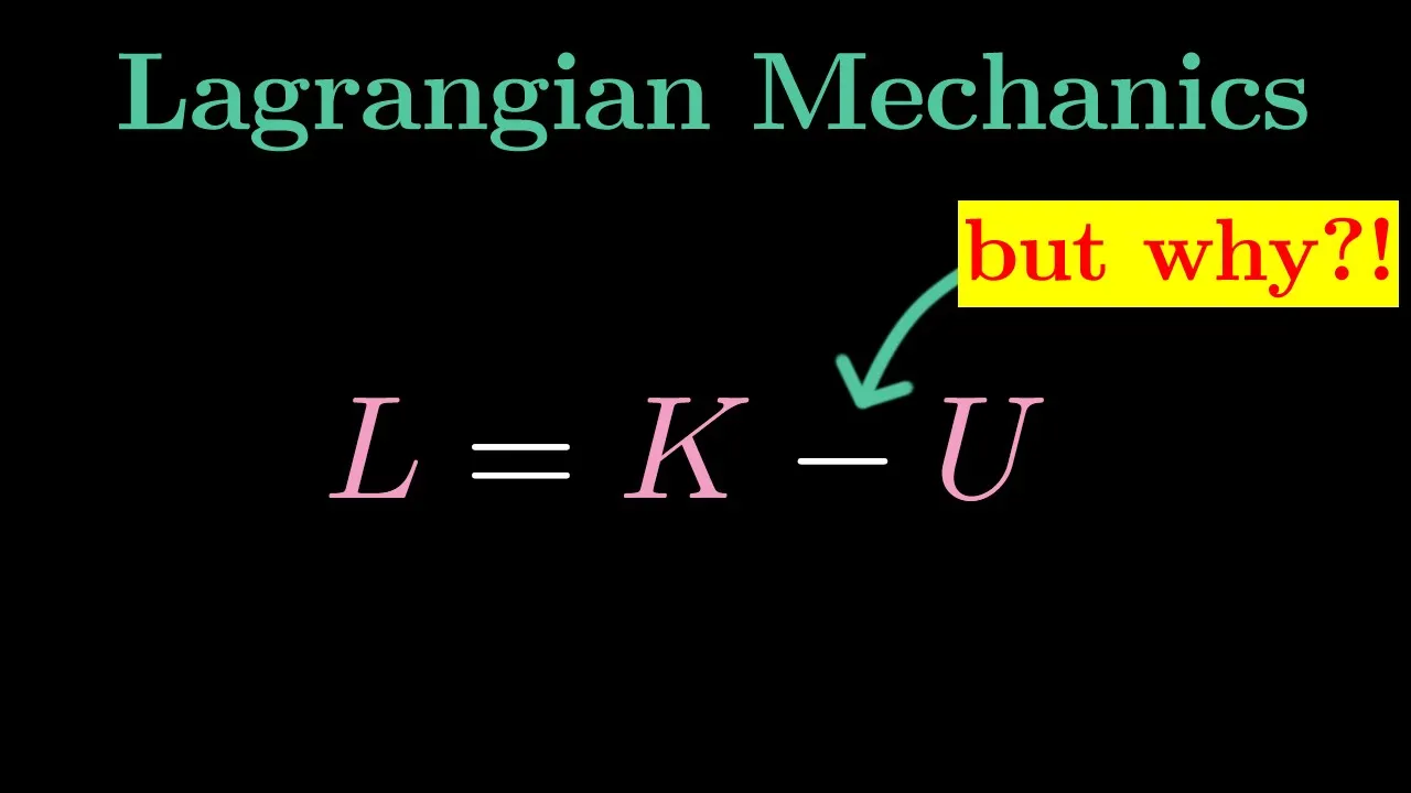

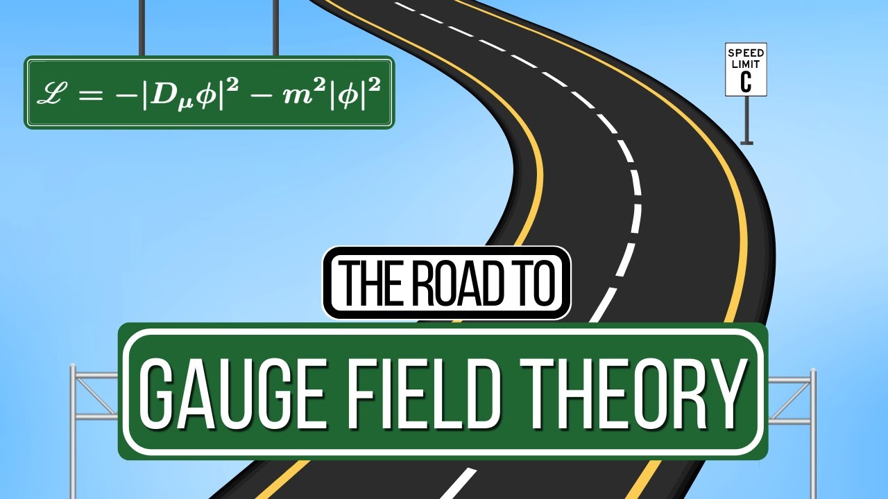











Lagrangian and Hamiltonian mechanics provide alternative mathematical frameworks to Newton's F=ma formulation for analyzing mechanical systems, where the Lagrangian L = T - V (kinetic minus potential energy) leads to the Euler-Lagrange equation d/dt(∂L/∂q̇) = ∂L/∂q, while the Hamiltonian H = T + V (total energy expressed in terms of coordinates and momenta) gives Hamilton's equations q̇ = ∂H/∂p and ṗ = -∂H/∂q, both yielding equivalent equations of motion but offering different analytical advantages such as easier handling of constraints and natural connections to quantum mechanics.
Classical Mechanics: Lagrangian and Hamiltonian Formulations
Added:Newton's Laws of Motion and classical Newtonian dynamics (force, mass, acceleration, and torque).
Calculus and differential equations, specifically partial derivatives and solving basic ordinary differential equations.
The concepts of kinetic energy (T) and potential energy (V) for conservative physical systems.
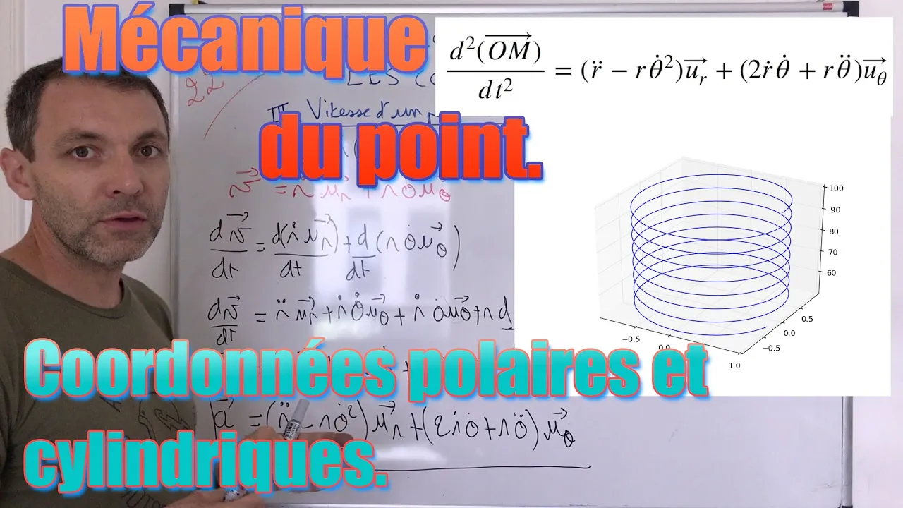
Coordinate systems and vector decomposition, particularly polar coordinates as applied to rotational or circular motion.
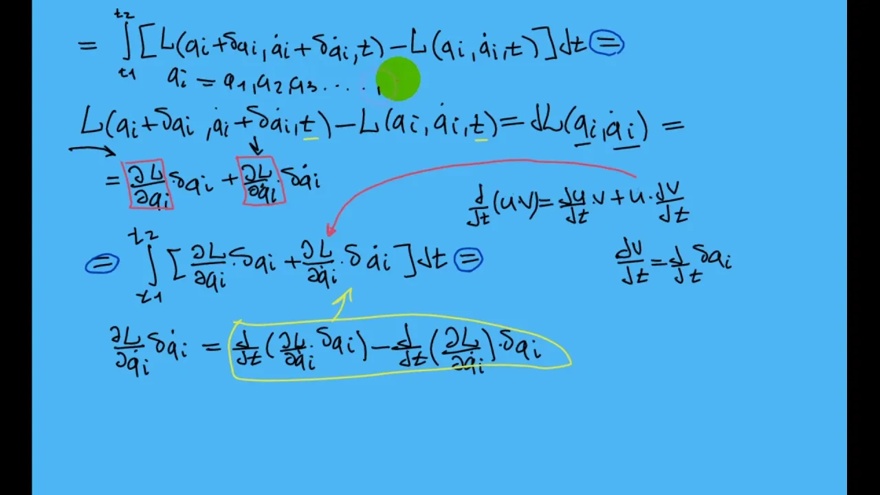
Hamilton's Principle and the Calculus of Variations, which form the mathematical foundation for deriving Lagrange's equations.
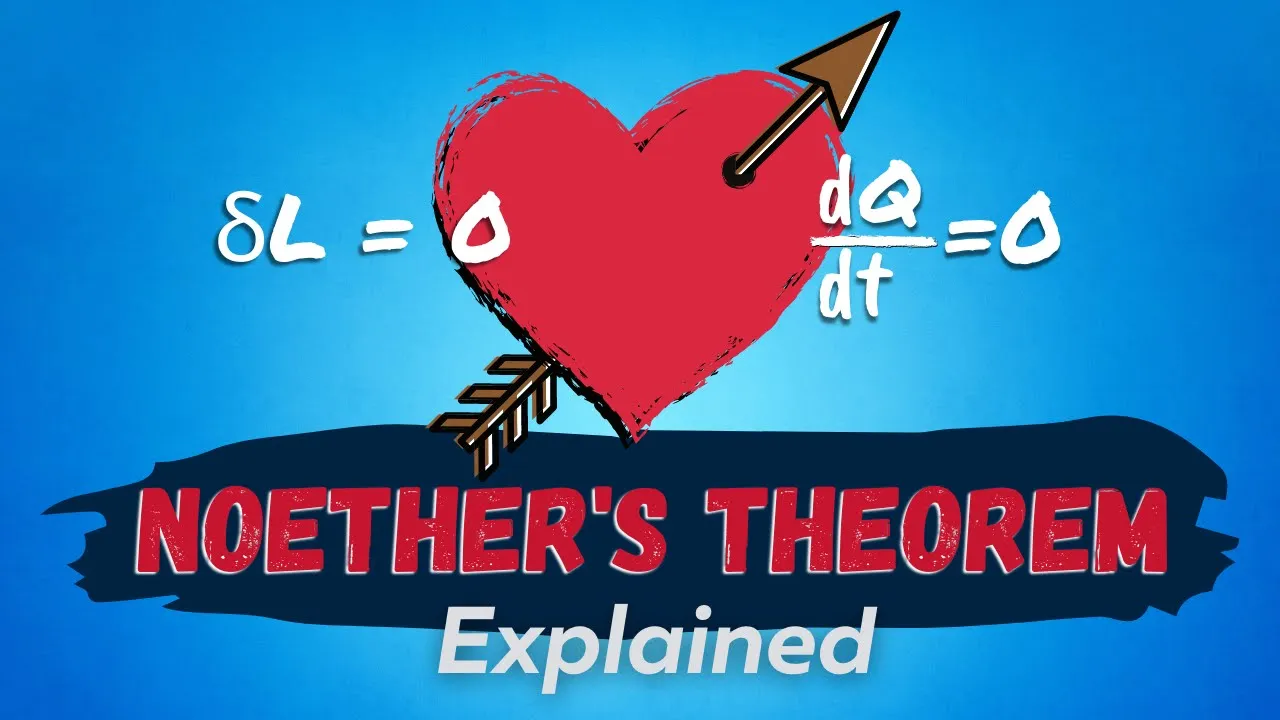
Noether's Theorem, exploring the profound connection between physical symmetries and conservation laws (e.g., energy, momentum).
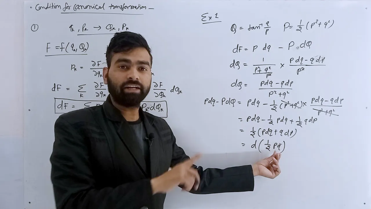
Canonical transformations and Poisson brackets, which are crucial for advanced theoretical formulations of classical mechanics.
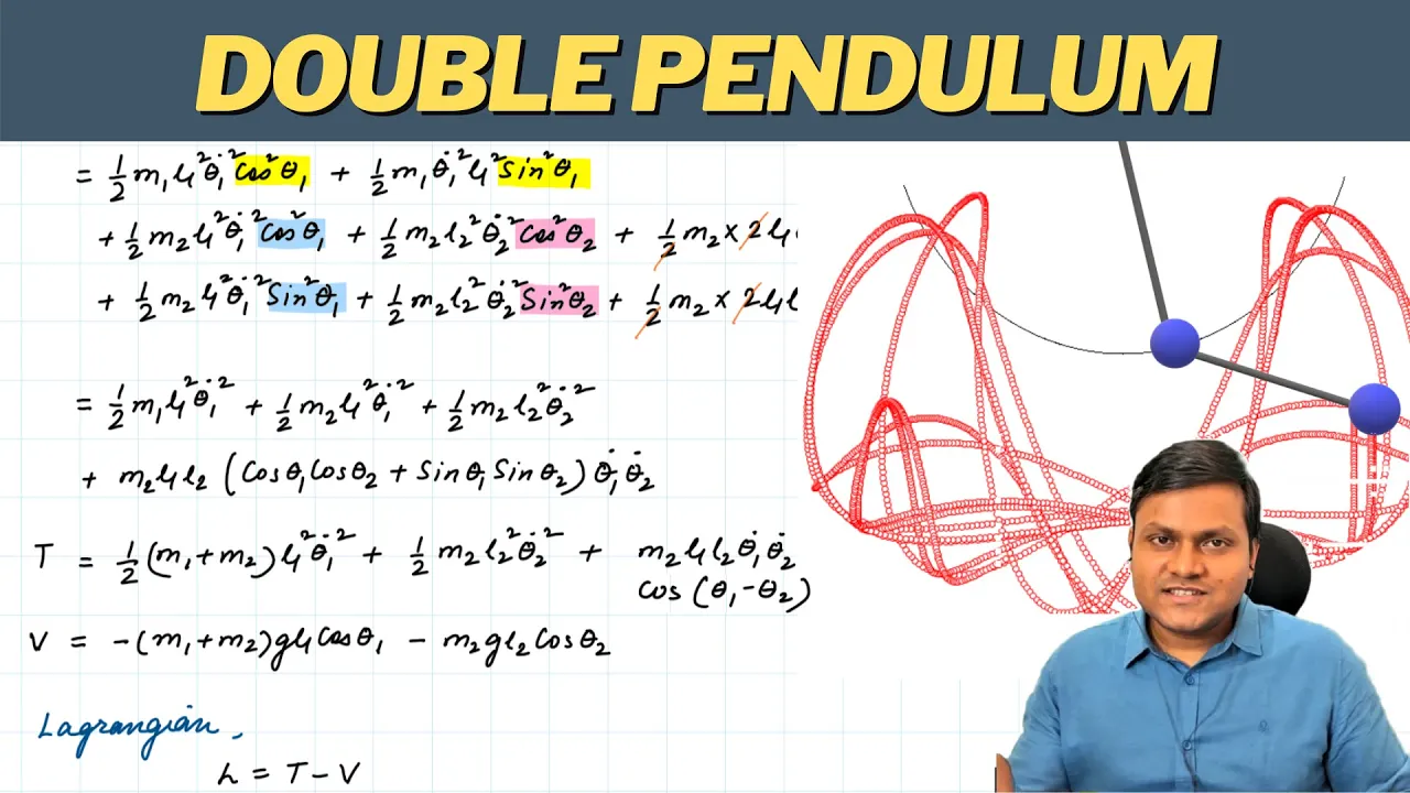
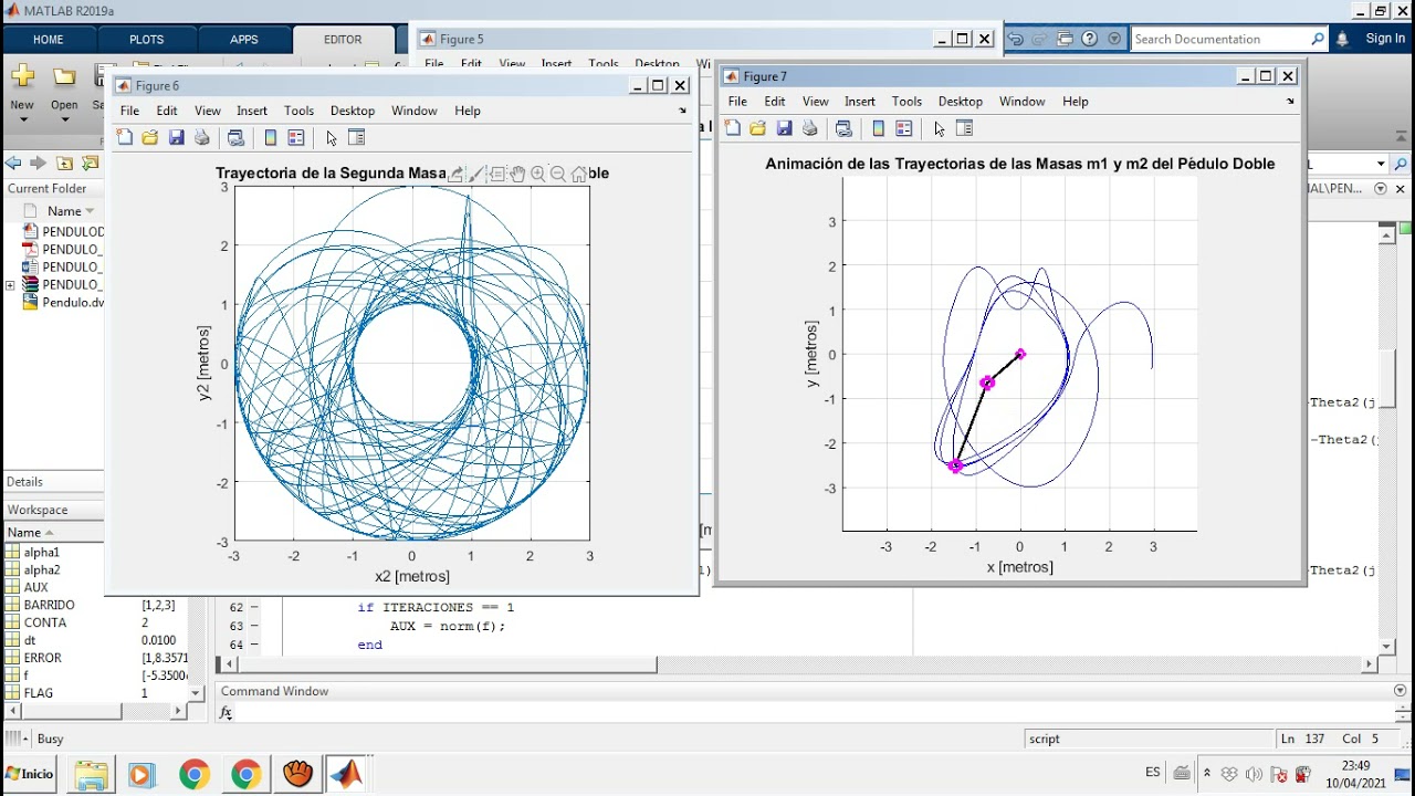
Chaotic systems and non-linear dynamics, such as analyzing the unpredictable motion of a double pendulum.
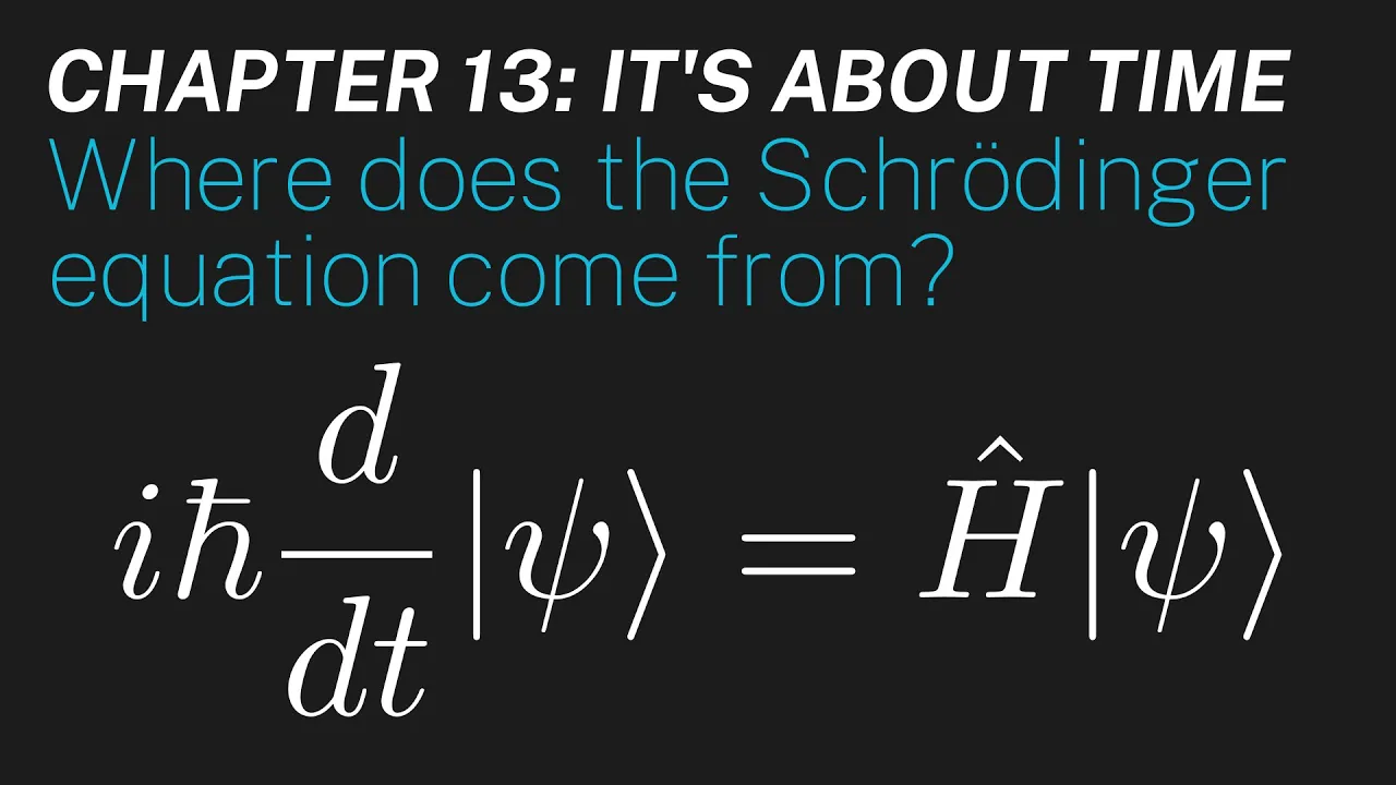
The transition to Quantum Mechanics, understanding how the Hamiltonian formulation maps onto quantum operators and the Schrödinger equation.
1.5M views42.2Klikes18:32Original Release: 2021-09-15
hello and welcome everybody my name is elliott and in this physics mini lesson i'm going to give you a quick introduction to the three formulations of classical mechanics aka newtonian lagrangian and hamiltonian mechanics newtonian mechanics is what everybody learns about in their first physics class when they learn to apply f equals ma to simple systems but there are two other formulations of mechanics that are actually more widely used by modern physicists and they're essential for understanding quantum mechanics meaning the physics of very small objects like elementary particles these are the lagrangian and hamiltonian formalisms of mechanics and in this video i'm going to teach you the basics of both i'm going to illustrate each approach using the simple pendulum as an example so we've got a particle of mass m hanging from a lightweight rod of length l which is attached to a pivot at its other end now i'll assume that you've already learned how to analyze a pendulum using f equals ma so i'm only going to review that briefly right now before i get into the lagrangian and hamiltonian approaches but i've posted a whole other video just reviewing the basics of pendulums that i'll link below so you can check that out if you want to see more of the details and i'll also paste a link to some notes that i wrote about these topics which you might also want to check out after you've watched this video first of all we need to set up some coordinates to describe the position of the pendulum we can use whatever coordinates we want but it's simplest to use either the arc length coordinate s that runs along the circumference of the circle traced out by the particle or we can use the angle that the rod makes with the vertical theta they're totally equivalent and either one will do the job for specifying the position of the mass the relation between them is just the definition of the angle theta in radians it's the arc length s divided by the radius l we want to predict how the pendulum is going to move when you pull it up to some initial angle and let it go or if you were to give it a little kick according to newton we should start by writing down all the forces that are acting on the particle there's only two of these gravity mg pointing straight down and the tension t in the rod pulling radially back toward the center of the circle then newton tells us to add up all the forces and write f equals ma the total force equals the mass times the acceleration f equals ma is a vector equation but what we're really interested in here is the tangential component meaning the component of the force and the acceleration that point along the circle where the particle is constrained to move the tension isn't contributing anything here that's pointing straight toward the center of the circle which is perpendicular to the tangent direction so the only relevant force is actually the tangential component of gravity with a little geometry work you can see this is mg sine theta pointing back toward the pendulum's equilibrium position so f equals ma for the arc length coordinate s simply reads m s double dot equals minus mg sine theta i'm using dots here to denote rates of change with respect to time so if s of t is the position as a function of time then s dot equals ds by dt is the velocity and s double dot is the acceleration the second derivative of s with respect to time i want to write everything in terms of theta though so i'm going to use the fact that s double dot is equal to l times theta double dot in order to rewrite the f equals ma equation as theta double dot equals minus g over l sine theta this is called the equation of motion for theta it's the differential equation that governs the motion of the pendulum and it's actually pretty complicated in this case because of this factor of sine theta on the right hand side too complicated in fact for us to be able to write down a simple solution in general there is one special case when we can though and that's when theta is small meaning that the pendulum never gets very far away from its equilibrium position in that case the solution is just a sine or cosine if you want to know how that works check out the other video that i posted all about pendulums that i've linked down below here's a little animation that i made to show you what this looks like i'll paste a link below so you can go play with it too you drag these little sliders here to set the initial angle and initial angular speed of the pendulum and then press start to let it go and see the resulting motion when i release it from a small angle like this you can see that theta versus t indeed looks like a cosine function so i hope you'll go play with this try choosing different values for the initial conditions by dragging those sliders draw for yourself what you think the graph of theta versus t should look like with those initial conditions and then press start to see if you got it right all right so that's a quick review of how we understand the motion of the pendulum using newtonian mechanics and f equals ma but there's a lot more to mechanics than f equals ma and in the years after newton's work in the late 1600s new approaches to mechanics were developed by joseph louis lagrange in the late 1700s and by william rowan hamilton in the 1800s lagrange and hamilton's approaches offer new practical and theoretical insights into the structure of mechanics and they're especially relevant in the study of quantum mechanics meaning the physics of very small objects like atoms and elementary particles as opposed to the classical mechanics that newton lagrange and hamilton originally studied now i should say that the lagrangian and hamiltonian approaches to mechanics are a little bit more mathematically sophisticated than newton's approach so depending on how much math you've already learned they might seem like they're a little bit more challenging but they're both really fascinating and they provide new insights and strategies for solving problems remember that it's also totally fine if you don't follow every single detail that i present here what i'm really hoping is that you'll be inspired to go off and keep learning more on your own alright let's look at the lagrangian formalism next whereas newton told us to start by writing down the total force lagrange tells us to start by writing down the kinetic energy the potential energy and then taking their difference this defines a function called the lagrangian l let's see what the lagrangian is for our pendulum example the kinetic energy k is of course just one half mv squared where v equals s dot is the speed of the particle actually i'd like to write everything in terms of theta so i'm going to replace s dot with l times theta dot then the kinetic energy is one half m l squared theta dot squared the potential energy u meanwhile is just mg times y the height of the particle above some chosen ground level i'm going to put ground level at the height of the pivot then the y coordinate of the particle is minus l cosine theta and the potential energy is minus mgl cosine theta so the lagrangian for our pendulum is the difference between the kinetic energy and potential energy that's one half m l squared theta dot squared plus mgl cosine theta so newton told us to start by writing the total force and setting it equal to m a lagrange instead tells us to start by writing the lagrangian like we have here and then using it to write what's called the euler lagrange equation that's d by dt of dl by d theta dot equals dl by d theta by the way the curly d's here stand for partial derivatives if you've never seen those before don't worry about it for practical purposes they behave just like ordinary derivatives now i'm not going to get into too much motivation as to where this euler lagrange equation comes from in this video what i just want to do for now is write it down and investigate the consequences but the short answer is that the euler lagrange equation is the condition for the action s to be minimized where the action is defined as the integral of the lagrangian the claim is that of all the possible paths that a particle could follow the one it actually chooses is the path that minimizes or more precisely extremizes the action this is known as the principle of least action and the implication is that the trajectory satisfies the oil and lagrange equation but unpacking all of those details would really require its own dedicated video right now i just want to see what happens when we plug the pendulum lagrangian into this euler lagrange equation the right hand side of the euler lagrange equation is the derivative of l with respect to theta and we're going to treat theta and theta dot as independent variables when we take these derivatives that means that the only contribution to dl by d theta comes from the cosine theta term in the lagrangian and we get dl by d theta equals minus mgl sine of theta for the left hand side we need to know what dl by d theta dot is and from the kinetic energy term we get ml squared theta dot then taking d by dt of that just turns theta dot into theta double dot by the way dl by d theta dot here is called the momentum p corresponding to the coordinate theta dl by d theta is called the generalized force the reason for the terminology is that the euler lagrange equation is then reminiscent of newton's second law force is the rate of change of momentum so the result of plugging in our pendulum lagrangian into the euler lagrange equation says that ml squared theta double dot equals minus mgl sine theta canceling out the common factors we once again obtain theta double dot equals minus g over l sine theta the same equation of motion we obtained earlier using f equals m a but this time we got it using a very different strategy based on the lagrangian and the euler lagrange equation all that might seem a little bit abstract if you've never encountered a lagrangian before but in fact it's a very useful way of quickly getting at the equations of motion for a system often times easier than using f equals ma if i'm faced with most any mechanics problem i'll usually start by writing down the lagrangian for one thing we don't have to deal with any of the annoying vectors that show up in f equals ma we can just choose whatever coordinates we like to describe our system including potentially non-inertial coordinates write down the lagrangian and then write the euler lagrange equation for each of the coordinates the lagrangian formalism also makes it much easier to deal with constraints and to understand symmetries but those topics will have to wait for another day now if you really want to master these ideas you've got to solve problems for yourself so i've posted a problem sheet down below where you can apply the lagrangian method to a challenging system it's our pendulum again this time in the guise of a pocket watch with magical powers and now the pivot is being shaken back and forth by a mysterious hypnotist that you bump into at the town fair so you should definitely go work that problem out to test and deepen your understanding and i've also posted a link to the solutions which are available on my website finally let's look at the pendulum using hamiltonian mechanics this time instead of starting with a lagrangian k minus u let's write down the total energy k plus u for the pendulum we get one half ml squared theta dot squared minus mgl cosine theta that minus sine is again there because the potential was negative now remember that we defined the momentum p by m l squared theta dot i'm going to use that expression to rewrite the first term and the energy as p squared over 2 m l squared that means we can write the total energy in terms of theta and p as p squared over 2 ml squared minus mgl cosine theta this quantity is called the hamiltonian and it's the starting point for hamiltonian mechanics just as the lagrangian was the starting point for lagrangian mechanics whereas we use the lagrangian to write down the euler lagrange equation we'll use the hamiltonian to write hamilton's equations which say that theta-dot equals the derivative of h with respect to p while p-dot is equal to minus the derivative of h with respect to theta note that whereas f equals m a and the euler lagrange equation gave us a single second order differential equation hamilton gives us a pair of first order equations for theta and p by the way it's important to mention here that while the hamiltonian was just the total energy in this simple example that's not always necessarily the case so let me give you the completely general definition before we move on remember that the momentum p was defined as the derivative of l with respect to the velocity the hamiltonian is defined by taking p times the velocity and then subtracting l and then as before you replace all the theta dots with p's now that may look like it comes out of left field and i don't have time to explain it right now but you can check that this definition reproduces the total energy in our pendulum example but in the system i ask you to solve on the problem sheet you're going to need this more general definition so let's see what we get for our simple pendulum the derivative of h with respect to p is just p over ml squared from the first term for the derivative with respect to theta we get minus sine theta from the derivative of cosine times two more minus sines gives us an overall minus mgl sine theta hamilton's equations tell us that p equals ml squared theta dot and p dot is equal to minus mgl sine theta this first equation is just the definition of momentum again if i take its rate of change it says that p dot equals ml squared theta double dot now if i insert that into hamilton's second equation we learned that ml squared theta double dot is equal to minus mgl sine theta crossing out the common factors we arrive one more time at our old friend theta double dot equals minus g over l sine theta so hamilton's equations are equivalent to the original equation of motion that we got either from f equals ma or from the euler lagrange equation they just split the single second order differential equation into a pair of first order equations first order because we only have one derivative acting on theta and p but what does that really buy us hamilton's pair of first order equations aren't necessarily any easier to solve than the single second order equation of motion that we started with what we do gain however is a new geometric perspective on the mechanics of the pendulum by connecting it to what's known as a flow on face space as i'll now explain to specify what the pendulum is doing at any given instant in time we just need to give its position and velocity or equivalently its position and momentum theta and p with this initial data we can figure out what the pendulum will be doing at any later time by solving hamilton's equations for theta of t and p of t the pairs of thetas and p's define a plane which is called the phase space of the system we start out at our initial condition theta of zero p of zero and as time goes on our coordinate moves around this theta p plane tracing out a curve which is known as a flow on this phase space these flows are very special they won't just travel along any old curve in the theta p plane in particular because the energy of the pendulum is conserved if we evaluate the hamiltonian at any time t along the flow we're guaranteed to always get the same number the energy is a constant of the flow here's what a few of the lines of constant energy look like for our pendulum because the energy of the pendulum is constant we know that our initial point has got to move along one of these lines of constant energy as it evolves with time so here's another little animation that i made again you drag these sliders to set the initial conditions that you want for the pendulum the initial conditions pick out your starting point in the face space so here i'm starting out with some particular angle and zero momentum then we're going to let the pendulum go and see how it evolves with time the pendulum moves its angle and angular velocity are changing with time and therefore the phase space coordinate is changing but since the energy is constant we know that the particle has got to travel along this line of constant energy so again i'll put a link to this little animation down below so that you can go play with it for yourself notice in particular that there are these two different kinds of curves of constant energy we've got these closed loops near the center of the face space and these open wavy lines farther away try setting the initial conditions so that the particle sits on one of the wavy lines and figure out what the physical difference is between these two types of phase space flows all this is only the tip of the iceberg for lagrangian and hamiltonian mechanics and i'm really hoping that i've wet your appetite to make you curious to go off and learn more for yourself not only are these fascinating and extremely useful approaches to classical mechanics they're also fundamental to the way we think about quantum mechanics for example functions on phase space and classical mechanics turn into operators on the quantum space of states in quantum mechanics and if you know the state of a quantum system at t equals 0 the schrodinger equation says that the state at a later time t will be e to the minus i over h bar h times t acting on the state where h is the operator version of the classical hamiltonian function so if you keep studying physics i guarantee you'll see lagrangians and hamiltonians popping up all over the place all right that's it for this video i really hope you found it interesting you can find all the links down in the description to the notes that i posted on my website to those animations and to the problem sheet and solutions please hit the like button subscribe to the channel to see more physics videos very soon and also leave me a comment to tell me what topics you might like to see me cover in the future thanks for watching everybody
Up Next

6:07
Lagrangian Mechanics: Why the Euler-Lagrange Equation Works
@MichelvanBiezen
187K views•2016-03-31

12:53
21cm Hyperfine Transition in Neutral Hydrogen: Radio Astronomy Basics
@AaronRobertParsons
12.4K views•2011-10-13

32:32
NMR Spin Physics I: Zeeman Effect, Resonance Condition & Larmor Frequency
@nptel-indianinstituteofsci8064
2.3K views•2024-01-17

27:14
Entropy and the Second Law of Thermodynamics Explained
@veritasium
27.5M views•2023-07-01
Related Study Plans & Knowledge Roadmaps
Structured learning paths in Physics
physics
Nuclear Physics (Decay, Fission & Reactors)
01Atomic Structure and the Binding Force
02Radioactive Decay and Half-Life
03Nuclear Fission Mechanics and Chain Reactions
+ 2 more learning modules
12h5 modules
Explore Roadmap
physics
Soft Matter (Polymers, Colloids & Rheology)
01Foundations of Soft Matter & Thermal Forces
02Polymer Physics and Macromolecules
03Colloids, Surfactants, and Self-Assembly
+ 2 more learning modules
38h5 modules
Explore Roadmap
physics
Analytical Mechanics: Lagrangian & Hamiltonian
01Mathematical Foundations: Calculus of Variations
02From Newtonian Mechanics to Constraint Dynamics
03The Principle of Least Action & Lagrangian Mechanics
+ 3 more learning modules
28h6 modules
Explore Roadmap
physics
General Relativity (Spacetime & Cosmology)
01Foundations of Relativity: Special Relativity
02The Geometry of Spacetime: Equivalence Principle & Curvature
03Einstein's Field Equations: The Mathematics of Gravity
+ 2 more learning modules
55h5 modules
Explore Roadmap