



















The Euler-Lagrange equation, derived from the Principle of Stationary Action, states that the true path of a physical system is found by setting the partial derivative of the Lagrangian with respect to position equal to the time derivative of the partial derivative of the Lagrangian with respect to velocity (d/dt(∂L/∂Ẋ) - ∂L/∂X = 0), meaning the actual path corresponds to a stationary point (not necessarily a minimum) of the Action functional, which is the integral of the Lagrangian over time.
Euler-Lagrange Equation Explained Intuitively | Lagrangian Mechanics
Added:Newtonian Mechanics: A solid grasp of Newton's laws of motion, kinetic energy, potential energy, and conservative forces.
Multivariable Calculus: Proficiency with partial derivatives, the chain rule, and total derivatives with respect to time.
Generalized Coordinates: Understanding how to describe a physical system's configuration using independent coordinates (q) rather than standard Cartesian coordinates.
Basic Calculus of Variations: Familiarity with the concept of a functional (a function of functions) and the goal of extremizing a path integral.
Hamiltonian Mechanics: Transitioning from Lagrangians to Hamiltonians using the Legendre transformation, and exploring Phase Space dynamics.
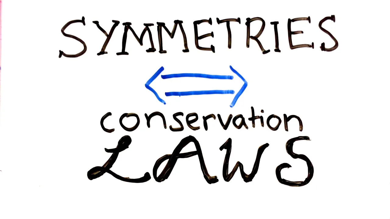
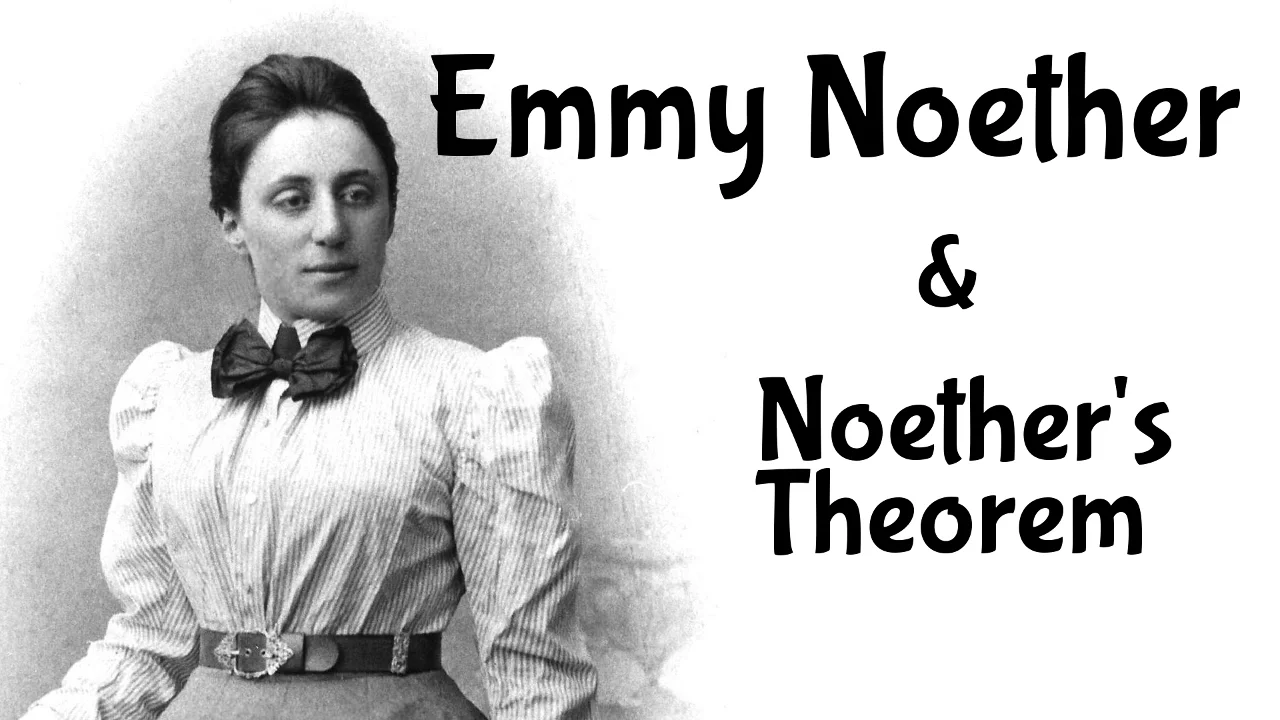
Noether's Theorem: Understanding the profound connection between continuous symmetries in a Lagrangian and physical conservation laws.
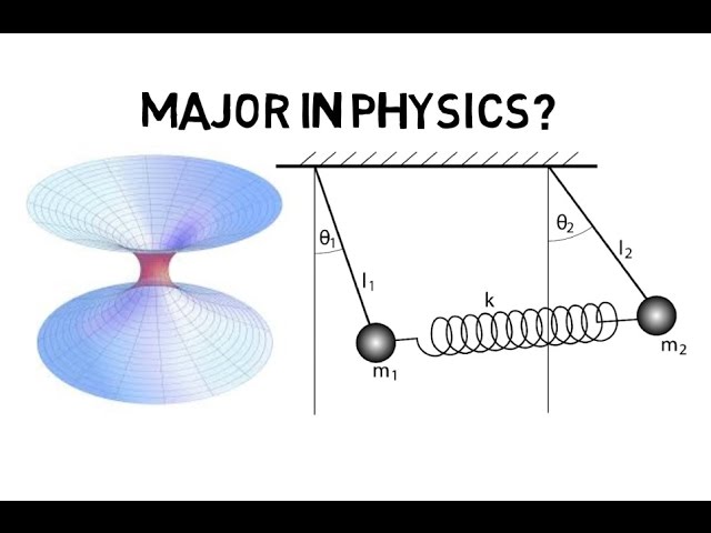
Advanced Classical Mechanics Applications: Applying the Euler-Lagrange equations to complex systems like the double pendulum, rigid body rotation, or systems with non-holonomic constraints.
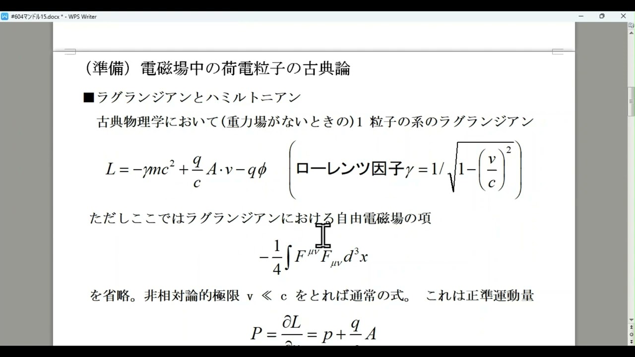
Lagrangian Field Theory: Extending the Euler-Lagrange equations from discrete particles to continuous fields, which is fundamental to classical electromagnetism and Quantum Field Theory.
444.8K views11.5Klikes18:22Original Release: 2018-11-18
In classical Newtonian physics, the Lagrangian of a system is the total kinetic energy minus the total potential energy.
In Quantum Field Theory, this simple relationship is no longer true, and the equation for the Lagrangian at each point in time is a function of all the fields throughout all of space.
We could be dealing with Einstein’s Theory of Relativity, or with Quantum Field Theory, or with Newton’s Laws of Motion.
When physicists propose new fundamental laws of physics, they often do so by proposing a new equation for the Lagrangian.
What we therefore want to focus on is not the equation for the Lagrangian in any one specific theory, but how the Lagrangian is used to predict the behavior of a system, as this has universal practical and philosophical importance.
Suppose we know the initial state and the final state of a system.
We wish to calculate the path between the initial and the final state.
The system can consist of any number of fields and particles, and the system can contain any number of independent variables.
Here, we just show three independent variables, which we will call “X”, “Y”, and “Z.” Let’s just show the variable X.
The variable X could refer to the position of a particle along one dimension.
In order to calculate the future behavior of a system, we need to know both the position and the velocity.
We will refer to the velocity in the X direction using the symbol X with a dot over it.
Suppose we have a function that depends on both the position and the velocity.
We will call this graph the Lagrangian.
The Lagrangian is also a function of all the other independent variables.
This graph could also be a function of time.
All the equations shown in this video will be valid regardless of whether or not the graph depends on time.
For the following animations, we will show a graph that does not change with time.
We don’t know the path between the initial and final state, but let us propose one possible path as a guess.
The height of the red ball at each point in time symbolizes the value of the Lagrangian at each point in time.
Here, the color symbolizes the value of the Lagrangian.
Time is not shown on this graph, but we can change the graph so that it shows the value of the Lagrangian as a function of time.
Let us say that the region in red is considered to have a “negative area” and the region in green is considered to have a “positive area.” The total area is what we will refer to as the “Action.” The “Action” is a function of the entire path as a whole.
If the path changes, then the “Action” also changes.
We can plot this on a graph as shown.
Let us consider the slope of this graph at each point.
If we are dealing with physical laws where the total work done depends only on the initial and final state of the system, and not on the path in between, then the true actual path of the system must be at a point where the slope of this graph is zero.
One place where the slope can be zero is where the Action is at a minimum.
For this reason, people often refer to using this method to find the path as the “Principle of Least Action.” However, a more accurate description would be the “Principle of Stationary Action”, since the actual path needs to be at a point where the slope of this blue line is zero.
To find where this happens, we need to consider the partial derivatives of the Lagrangian.
The slope of this line is the partial derivative of the Lagrangian with respect to X.
Here, the color represents the partial derivative of the Lagrangian with respect to X.
Let’s change the color of each ball to match the color of the graph at the ball’s location.
Let us now view this as a function of time.
Let’s change the vertical position of each ball based on its color.
We now have as a function of time, the partial derivative of the Lagrangian with respect to X.
This is just one of the partial derivatives we can have.
We can also have the partial derivative of the Lagrangian with respect to the variable symbolized by the X with the dot over it, which we well call “X dot.” Here, the color represents the partial derivative of the Lagrangian with respect to “X dot.” Let’s change the color of each ball to match the color of the graph at the ball’s location.
Let us view this as a function of time.
Let’s change the vertical position of each point based on its color.
We now have as a function of time, the partial derivative of the Lagrangian with respect to “X dot.” Let us represent the slope of this function of time with a new set of colors.
Let’s again change the vertical position of each point based on its new color.
We now have this new expression as a function of time.
We are now ready to use these expressions to find the path of the system.
Consider the following expression.
For the slope of the blue line to be zero, this expression must also be equal to zero.
Let’s get an intuitive understanding of why this must be true.
The slope of the blue line being zero means that the “Action” will stay about the same for any exceedingly small change in the path.
Let us consider a simple example.
Suppose we make a small change in the path by moving just one of the red points.
The amount by which the Lagrangian will change for this point is equal to the partial derivative of the Lagrangian with respect to X.
Therefore, the amount by which the Action will increase is also equal to this amount.
Consider how the velocity of this curve has changed.
The velocity of this curve is represented by “X dot.” Therefore, these two other red points must move as shown.
Here, the Lagrangian for one point goes up, and the Lagrangian of the other point goes down by an equal amount, resulting in no net change in the total Action.
But, let’s now consider a case where the partial derivative of the Lagrangian with respect to “X dot” is not the same at these two points.
Now both of the points will go down, resulting in a decrease in the total action.
The decrease in the action is the rate at which the partial derivative of the Lagrangian with respect to “X dot” is changing with time.
Therefore, the total change in action is equal to the equation we saw earlier.
If this equation is equal to zero, then this means that the change in action is zero for any exceedingly small change in the path.
And this happens only for cases where the slope of the blue line is zero, which must be the case for the true actual path.
The variable “X dot” represents the partial derivative of the variable X with respect to time.
For the true actual path, this equation must also be true for any independent variable of the system, and there is no limit to how many independent variables a system can have.
If we are dealing with quantum field theory, we will have a variable representing each of the fields throughout all of space, and we have to take into account not just the partial derivatives with respect to time, but also the partial derivatives with respect to each of the spatial dimensions.
Here, the initial and final conditions are the quantum fields throughout all of space at two different points in time, and the equation below must be zero for the description of how each quantum field evolves through time.
But visualizing Quantum Field Theory is a topic for another video.
Up Next
18:32
Classical Mechanics: Lagrangian and Hamiltonian Formulations
@PhysicswithElliot
1.5M views•2021-09-15

12:53
21cm Hyperfine Transition in Neutral Hydrogen: Radio Astronomy Basics
@AaronRobertParsons
12.4K views•2011-10-13
12:39
Quarks, Gluons, and the Strong Nuclear Force: QCD Explained
@EugeneKhutoryansky
478K views•2018-07-07

27:14
Entropy and the Second Law of Thermodynamics Explained
@veritasium
27.5M views•2023-07-01
Related Study Plans & Knowledge Roadmaps
Structured learning paths in Physics
physics
Nuclear Physics (Decay, Fission & Reactors)
01Atomic Structure and the Binding Force
02Radioactive Decay and Half-Life
03Nuclear Fission Mechanics and Chain Reactions
+ 2 more learning modules
12h5 modules
Explore Roadmap
physics
Soft Matter (Polymers, Colloids & Rheology)
01Foundations of Soft Matter & Thermal Forces
02Polymer Physics and Macromolecules
03Colloids, Surfactants, and Self-Assembly
+ 2 more learning modules
38h5 modules
Explore Roadmap
physics
Analytical Mechanics: Lagrangian & Hamiltonian
01Mathematical Foundations: Calculus of Variations
02From Newtonian Mechanics to Constraint Dynamics
03The Principle of Least Action & Lagrangian Mechanics
+ 3 more learning modules
28h6 modules
Explore Roadmap
physics
General Relativity (Spacetime & Cosmology)
01Foundations of Relativity: Special Relativity
02The Geometry of Spacetime: Equivalence Principle & Curvature
03Einstein's Field Equations: The Mathematics of Gravity
+ 2 more learning modules
55h5 modules
Explore Roadmap