Academic Databases
Explore Our Semantic Databases
STEM & Tech
Math, Physics, CS & Engineering...
Economics
Macro, Micro, Econometrics...
Business
Management, Marketing, Finance...
Health & Life Sciences
Biology, Medicine, Neuroscience...
Humanities & Social Sciences
Psychology, Law, Philosophy, History...
General Studies
General & interdisciplinary studies...
Explore Topics
Features

Solving Hamilton-Jacobi Equation via Separation of Variables

Added: 2026-08-14

Deep Dive

Fundamentals of Hamiltonian Mechanics, including the definition of the Hamiltonian, generalized coordinates, and Hamilton's equations of motion.

PGTRB PHYSICS -HAMILTONS EQUATIONS

PGTRB PHYSICS -HAMILTONS EQUATIONS

468

The Hamiltonian function H is defined as H = Σ(p_j * q̇_j) - L, where L is the Lagrangian. Unlike Lagrangian mechanics which depends only on coordinates and time, the Hamiltonian depends on coordinates, momenta, and time. Hamilton's equations are first-order differential equations, in contrast to Lagrange's second-order equations. For n particles, Lagrangian mechanics requires 3n coordinates and 3n second-order equations, while Hamiltonian mechanics requires 6n first-order equations (3n for coordinates and 3n for momenta).

Click to watch →

Hamilton's equation of motion#Hamilton's canonical eqns#Classical mechanics#Hamiltonian formulation#

Hamilton's equation of motion#Hamilton's canonical eqns#Classical mechanics#Hamiltonian formulation#

10.6K

This section establishes the mathematical foundations for Hamiltonian mechanics. The Hamiltonian function H is defined as a function of generalized coordinates QJ, generalized momenta PJ, and time T. The chain rule for functions of multiple variables provides the mathematical framework for taking differentials: dF = (∂F/∂u)du + (∂F/∂v)dv. The Lagrangian function L is introduced as depending on generalized coordinates QJ, generalized velocities QJ dot, and time T. Key relationships are established: generalized momenta PJ = ∂L/∂QJ dot and their time derivatives PJ dot = ∂L/∂QJ. These definitions and relationships form the essential vocabulary and mathematical machinery needed to derive Hamilton's canonical equations.

Click to watch →

(Lec 15) Hamilton's Equations of Motion | Hamiltonian | PROBLEM SOLVING

(Lec 15) Hamilton's Equations of Motion | Hamiltonian | PROBLEM SOLVING

21.4K

Hamiltonian mechanics provides an alternative framework to Lagrangian mechanics for analyzing mechanical systems. The framework uses generalized coordinates (q_i) representing degrees of freedom, generalized velocities (q̇_i), and generalized momenta (p_i = ∂L/∂q̇_i). The Hamiltonian (H) is obtained through Legendre transformation: H = Σ(p_i q̇_i) - L. Hamilton's equations of motion consist of three fundamental equations: (1) q̇_i = ∂H/∂p_i (velocity-momentum relation), (2) ṗ_i = -∂H/∂q_i (equation of motion), and (3) dH/dt = -∂L/∂t (energy conservation). When the Lagrangian is not explicitly time-dependent and the potential is velocity-independent, the Hamiltonian equals the total energy (H = T + V). For a spring-mass system with mass m and spring constant k, the Lagrangian is L = (1/2)mẋ² - (1/2)kx², the canonical momentum is p = mẋ, and the Hamiltonian is H = p²/(2m) + (1/2)kx². Using Hamilton's equations yields the standard harmonic oscillator equation mẍ + kx = 0, with solution x(t) = A cos(ωt + φ) where ω² = k/m. The third Hamilton equation confirms energy conservation when L has no explicit time dependence.

Click to watch →

[해밀턴 역학] 1. 해밀토니안, 운동 방정식

[해밀턴 역학] 1. 해밀토니안, 운동 방정식

8.7K

Hamiltonian mechanics is an alternative formulation of classical mechanics that uses the Hamiltonian function (H), obtained through Legendre transformation from the Lagrangian (L), to describe the dynamics of physical systems. The Hamiltonian is defined as H = Σ(p_k * q̇_k) - L, where p_k are the generalized momenta (p_k = ∂L/∂q̇_k) and q_k are the generalized coordinates. Hamilton's equations of motion are: q̇_k = ∂H/∂p_k and ṗ_k = -∂H/∂q_k. Physically, the Hamiltonian represents the total energy of the system (H = T + V), while the generalized momenta correspond to the system's momenta (p = mv for simple systems). These equations provide a complete description of the system's evolution in terms of position and momentum variables.

Click to watch →

Смотрим термех и гравитациюDX

Смотрим термех и гравитациюDX

724

This segment introduces Hamiltonian mechanics and Hamilton's equations. The Hamiltonian H is defined as H = Σ(q̇_i ∂L/∂q̇_i) - L. For a system with L = (1/2)Σm_i v_i² - V(q), the Hamiltonian is H = (1/2)Σp_i²/m_i + V(q), which is the total energy. Hamilton's equations are: q̇_i = ∂H/∂p_i, ṗ_i = -∂H/∂q_i. These equations are equivalent to the Euler-Lagrange equations but are first-order differential equations. For a system with L = (1/2)Σm_i v_i² - V(q), Hamilton's equations are q̇_i = p_i/m_i, ṗ_i = -∂V/∂q_i.

Click to watch →

Deep Dive

The concept of Canonical Transformations and Generating Functions, specifically how they relate to Hamilton's Principal Function.

تسجيل2 Ch9 2

تسجيل2 Ch9 2

923

Canonical transformations preserve Hamilton's principle and the structure of Hamiltonian mechanics. Four types of generating functions (F₁, F₂, F₃, F₄) facilitate coordinate and momentum transformations. F₁ depends on old coordinates and new coordinates, yielding p = ∂F₁/∂q and P = -∂F₁/∂Q. F₂ depends on old coordinates and new momenta, yielding p = ∂F₂/∂q and Q = ∂F₂/∂P. F₃ depends on old momenta and new coordinates, yielding q = -∂F₃/∂p and P = ∂F₃/∂Q. F₄ depends on old and new momenta, yielding q = -∂F₄/∂p and Q = -∂F₄/∂P. For all types, the new Hamiltonian K equals H + ∂F/∂t. These transformations allow solving for coordinates and momenta as functions of each other and time, essential for simplifying Hamiltonian systems.

Click to watch →

Classical Mechanics - Hamilton-Jacobi Theory : H-J Equation / Hamilton’s Principal Function

Classical Mechanics - Hamilton-Jacobi Theory : H-J Equation / Hamilton’s Principal Function

14.1K

The Hamilton-Jacobi equation is a first-order partial differential equation derived from canonical transformations where both the new coordinates and momenta are cyclic (not appearing explicitly in the Hamiltonian), and it is given by ∂S/∂t + H(q, ∂S/∂q, t) = 0, where S (Hamilton's Principal Function) is the generating function of the canonical transformation and represents the time integral of the Lagrangian (action) of the system.

Click to watch →

Canonical Transformations & Hamilton-Jacobi Method (Math Heavy) - Goldstein Ch 9, 10

Canonical Transformations & Hamilton-Jacobi Method (Math Heavy) - Goldstein Ch 9, 10

2.7K

A canonical transformation is a process for transforming any set of valid canonical coordinates and their conjugate momenta into any other valid set. This is achieved using generating functions, which are mathematical tools with no physical interpretation. There are four types of generating functions (F1-F4) based on their variable dependencies. The process involves either using a known generating function to find new coordinates and momenta, or using a known coordinate transformation to derive the generating function. The Hamiltonian transformation equation, derived from the least action principle, provides the mathematical foundation for these transformations.

Click to watch →

8 - 3 - The Hamilton-Jacobi Equation

8 - 3 - The Hamilton-Jacobi Equation

4K

Canonical transformations preserve Hamilton's equations through coordinate changes in phase space. A point transformation defines new coordinates Q_j as functions of original coordinates q_i, their momenta p_i, and time. Generating functions provide the mathematical framework: adding the time derivative of any function f(q, Q, t) to the Lagrangian preserves equations of motion. Four basic generating function types exist: F1(q, Q, t), F2(q, P, t), F3(p, Q, t), and F4(p, P, t). Each type yields specific transformation rules connecting old and new canonical variables through partial derivatives, enabling systematic exploration of equivalent mechanical descriptions.

Click to watch →

Hamilton-Jacobi Theory | Canonical Transformations and Solving Hamiltonian Systems (Lecture 9)

Hamilton-Jacobi Theory | Canonical Transformations and Solving Hamiltonian Systems (Lecture 9)

30.8K

Taking the total derivative of s(q, Q̃, t) gives ds/dt = Σp_i q̇_i + ∂s/∂t. Using p_i = ∂s/∂q_i and q̇_i = ∂H/∂p_i, and knowing that H + ∂s/∂t = 0, we find ds/dt = L, where L is the Lagrangian. Therefore, Hamilton's principal function differs from the action integral by at most an additive constant, justifying the notation s for action.

Click to watch →

Deep Dive

Basic proficiency in solving Partial Differential Equations (PDEs), particularly using the technique of additive separation of variables.

separation of variables شرح

separation of variables شرح

18.3K

The basic separation of variables technique for PDEs involves assuming a solution of the form u(x,y) = X(x)Y(y). Substituting into the PDE and dividing by X(x)Y(y) separates the equation into terms depending only on x and terms depending only on y. Each side is then set equal to a constant (separation constant), resulting in ordinary differential equations for each variable.

Click to watch →

Part-5 || Solution of Partial Differential Equation Using Method of Separation of Variables || PDE

Part-5 || Solution of Partial Differential Equation Using Method of Separation of Variables || PDE

1.2K

The Method of Separation of Variables is a technique for solving Partial Differential Equations (PDEs) by assuming the solution can be written as a product of functions, each depending on only one independent variable. This method transforms the PDE into ordinary differential equations (ODEs) that can be solved separately. The general approach involves: (1) assuming a separable solution form, (2) substituting into the PDE, (3) separating variables so that each side depends on only one variable, (4) equating both sides to a constant (separation constant), and (5) solving the resulting ODEs. This method is particularly useful for linear PDEs with homogeneous boundary conditions, such as the heat equation, wave equation, and Laplace equation.

Click to watch →

#19 Method of Separation of Variable | P.D.E. | CVPD | GTU

#19 Method of Separation of Variable | P.D.E. | CVPD | GTU

40.4K

The Method of Separation of Variables is a fundamental technique for solving Partial Differential Equations (PDEs) by assuming the solution can be expressed as a product of functions, each depending on only one independent variable. This method transforms the PDE into a set of ordinary differential equations (ODEs) that can be solved independently. The general procedure involves: (1) assuming a separable solution form, (2) substituting into the PDE, (3) rearranging terms to separate variables, (4) setting each side equal to a constant (separation constant), and (5) solving the resulting ODEs. This technique is particularly effective for linear PDEs with homogeneous boundary conditions and is widely used in physics and engineering applications such as heat conduction, wave propagation, and quantum mechanics.

Click to watch →

31. Method of Separation of Variables | Complete Concept & Problem#3 | PDE | Most Important

31. Method of Separation of Variables | Complete Concept & Problem#3 | PDE | Most Important

85.3K

The separation of variables method is a technique for solving partial differential equations by assuming the solution can be written as a product of functions, each depending on only one independent variable. For the PDE ∂u/∂x + ∂u/∂y = 3u, we assume u(x,y) = X(x)Y(y). Substituting this into the PDE gives X'(x)Y(y) + X(x)Y'(y) = 3X(x)Y(y). Dividing both sides by X(x)Y(y) yields X'(x)/X(x) + Y'(y)/Y(y) = 3. Since the left side depends only on x and the right side only on y, both must equal a constant (separation constant).

Click to watch →

Separação de Variáveis 1 - Introdução

Separação de Variáveis 1 - Introdução

3.7K

Separation of variables is a fundamental technique for solving partial differential equations (PDEs). Unlike ordinary differential equations, not all PDEs can be solved using this method, but a significant number can. Three common PDEs solvable by this method are Laplace's equation (∇²u = 0), the heat equation (∂u/∂t = α∂²u/∂x²), and the wave equation (∂²u/∂t² = c²∂²u/∂x²). Laplace's equation describes steady-state phenomena and is time-independent, while the heat and wave equations are time-dependent. The core assumption is that the solution can be expressed as a product of functions, each depending on only one variable (e.g., u(x,t) = X(x)T(t)). This transforms a PDE into simpler ordinary differential equations (ODEs). The procedure involves assuming a separable form, substituting into the PDE, verifying separation, solving the resulting ODEs, reconstructing the solution, and for parameter-dependent cases, expressing the general solution as a series (typically Fourier series) to satisfy boundary and initial conditions.

Click to watch →

Deep Dive

The physical setup of a particle in a uniform gravitational field, including its potential and kinetic energy formulations in Cartesian coordinates.

IndVirtu | Mekanika Analitik (Bagian 3)

IndVirtu | Mekanika Analitik (Bagian 3)

610

For a particle of mass m in a uniform gravitational field near Earth's surface, the configuration space is R³. The kinetic energy is T = (1/2)m(ẋ² + ẏ² + ż²) and the potential energy is V = mgz (with z = 0 at the reference level). The Lagrangian is L = (1/2)m(ẋ² + ẏ² + ż²) - mgz. Applying the Euler-Lagrange equations gives three equations of motion: mẍ = 0, mÿ = 0, and mż̈ = -mg. These describe free fall under gravity: the particle accelerates downward with acceleration g while maintaining constant velocity in the horizontal directions.

Click to watch →

AULA 12_ Turma 66_ Aplicações2_ Mec.Lagrangeana

AULA 12_ Turma 66_ Aplicações2_ Mec.Lagrangeana

416

For a free particle in Cartesian coordinates, the kinetic energy is T = (1/2)m(ẋ² + ẏ²), where ẋ and ẏ are the time derivatives of the Cartesian coordinates. The potential energy for a particle in a gravitational field is V = mgy. Since x and y are independent coordinates, they serve as the generalized coordinates for the system. The velocity vector is ẋî + ẏĵ, and the speed squared is ẋ² + ẏ².

Click to watch →

31.Mechanics:Hamilton's Equations in Cartesian coordinate system with potential

31.Mechanics:Hamilton's Equations in Cartesian coordinate system with potential

5.2K

For a particle moving in space under a conservative force field with potential V, the Hamiltonian is given by H = (p_x² + p_y² + p_z²)/(2m) + V(x,y,z), where p_x = mẋ, p_y = mẏ, and p_z = mż are the canonical momenta. Hamilton's equations for this system are: ṗ_x = -∂V/∂x, ṗ_y = -∂V/∂y, ṗ_z = -∂V/∂z, and ẋ = p_x/m, ẏ = p_y/m, ż = p_z/m. These equations reduce to Newton's second law when applied to gravitational potential V = mgz, yielding ẍ = 0, ẏ = 0, and ẑ = -g, which describes free fall under constant gravitational acceleration.

Click to watch →

Mechanics I Lecture #15 Module 2.4

Mechanics I Lecture #15 Module 2.4

1K

For uniform gravitational field F = -mg k̂, potential energy is U(z) = mgz (with U=0 at reference point). The energy method solves projectile motion efficiently: initial kinetic energy equals final kinetic plus potential energy. Starting from ground level, ½mv² = ½mv_H² + mgH, giving v_H = √(v² - 2gH). This handles all three dimensions simultaneously, avoiding separate equations of motion.

Click to watch →

Cursos Unicamp: Física Geral 1 / aula 13

Cursos Unicamp: Física Geral 1 / aula 13

105.4K

In a uniform gravitational field near Earth's surface, the gravitational potential energy difference between two heights y₁ and y₂ is ΔU = mgΔh, where Δh = y₂ - y₁. The formula U = mgy is derived by choosing the reference point at y = 0 where U = 0. The choice of reference point is arbitrary since only differences in potential energy matter for physical predictions.

Click to watch →

Hamilton-Jacobi Setup

Separation of Variables

Solving for Components

Deriving Momenta

Finding Q1 and Q2

Canonical Transformations

Equations of Motion

Hamilton-Jacobi Setup

0:00

Playing Section

1
Defines the Hamiltonian for a particle in a uniform gravitational field.
2
State the Hamilton-Jacobi equation and substitute momenta with partial derivatives of S.

Deep Dive

Applying the Hamilton-Jacobi equation to more complex physical systems, such as the Kepler/central force problem or the multi-dimensional harmonic oscillator.

MSC PRE PHYSICS - CLASSICAL MECHANICS - SOLUTION OF KEPLER PROBLEM BY HAMILTON JACOBI METHOD (1)

MSC PRE PHYSICS - CLASSICAL MECHANICS - SOLUTION OF KEPLER PROBLEM BY HAMILTON JACOBI METHOD (1)

722

This section establishes the Hamiltonian framework for solving Kepler's problem. The Hamilton-Jacobi equation H + ∂S/∂t = 0 is introduced, where H is the Hamiltonian and S is Hamilton's principal function. For a particle of mass m under inverse square central force F = -k/r², the potential energy is V = -k/r. The kinetic energy in polar coordinates is T = (1/2)m(ṙ² + r²θ̇²). The Hamiltonian is H = T + V = (1/2m)(pᵣ² + pθ²/r²) - k/r. For conservative systems, H equals total energy E. The Hamilton-Jacobi method introduces a generating function W(r, θ) with transformation equations pᵣ = ∂W/∂r and pθ = ∂W/∂θ, leading to the Hamilton-Jacobi equation (1/2m)[(∂W/∂r)² + (1/r²)(∂W/∂θ)²] - k/r = E.

Click to watch →

A way to understand the Kepler problem via the Hamilton-Jacobi formalism

A way to understand the Kepler problem via the Hamilton-Jacobi formalism

115

This section covers the complete application of the Hamilton-Jacobi formalism to solve the Kepler problem. The Hamiltonian for the Kepler problem in parabolic coordinates is H = (1/2m)(p_u² + p_v²/(u² + v²)) - 2k/(u² + v²). The Hamilton-Jacobi equation H(q, ∂S/∂q, t) + ∂S/∂t = 0 is applied with the ansatz S = A(u) + B(v) - Et, where E is the energy constant. Through separation of variables and algebraic manipulation, the method reduces the partial differential equation to ordinary differential equations for A(u) and B(v), demonstrating how the Hamilton-Jacobi approach systematically solves classical mechanical problems.

Click to watch →

理論物理学入門Ⅱ古典力学23

理論物理学入門Ⅱ古典力学23

100

This lecture demonstrates solving the Hamilton-Jacobi equation for a harmonic oscillator, deriving the action variable J = 2πE/ω and angle variable W = ωt + β, then applies the same method to the Kepler problem to express orbital parameters (semi-major axis and eccentricity) in terms of action variables, and finally solves the hydrogen molecule problem using elliptic-cylindrical coordinates (λ, μ) where λ = (R₁ + R₂)/2 and μ = (R₁ - R₂)/2, showing how the Hamilton-Jacobi method simplifies complex mechanical systems by separating variables and finding the principal function S.

Click to watch →

Уравнение Гамильтона-Якоби (все что нужно о нем знать)

Уравнение Гамильтона-Якоби (все что нужно о нем знать)

1.7K

For a particle in polar coordinates with Hamiltonian H = pr²/(2m) + pφ²/(2mr) + U(r), the Hamilton-Jacobi equation is ∂S/∂t + pr²/(2m) + pφ²/(2mr) + U(r) = 0. Since φ is cyclic, separate variables as S = -Et + pφφ + S_r(r). The reduced equation for S_r(r) is -E + (1/2m)(dS_r/dr)² + pφ²/(2mr) + U(r) = 0. Solving this ODE determines S_r(r), from which r(t) is found. Differentiating S with respect to pφ gives φ = φ₀ (constant), while differentiating with respect to pr gives pr = pr(t). This completely determines the motion, demonstrating how the Hamilton-Jacobi method systematically solves central force problems.

Click to watch →

Hamilton-Jacobi Theory | Canonical Transformations and Solving Hamiltonian Systems (Lecture 9)

Hamilton-Jacobi Theory | Canonical Transformations and Solving Hamiltonian Systems (Lecture 9)

30.8K

For time-independent Hamiltonians (∂H/∂t = 0), the generating function simplifies to s = w(q, Q̃) - Et, reducing the equation to H(q, ∂w/∂q, t) = E. Taking the total derivative reveals ds/dt = L, showing Hamilton's principal function differs from the action integral by an additive constant. For central force problems in polar coordinates, the kinetic energy is T = p_r²/(2m) + p_θ²/(2mr²). Multiplying the Hamilton-Jacobi equation by 2mr² enables separation of variables: r²[(∂²w/∂r²) + (1/r)(∂w/∂r)] - (2mV(r)r² - 2mEr²) = -∂²w/∂θ². Setting each side equal to a constant (-q₂²) yields independent equations. The angular equation integrates to w_θ(θ) = q₂θ + C, while the radial equation becomes √[2m(E - V(r)) - q₂²/r²] dr = ±√(2m) dr.

Click to watch →

Deep Dive

Introduction to Action-Angle Variables, which are crucial for analyzing periodic and quasi-periodic mechanical systems without fully solving the equations of motion.

Action Angle Variables - Lecture 1

Action Angle Variables - Lecture 1

3.3K

Action angle variables provide a method to find the period or frequency of periodic systems without finding the complete solution; the action variable J is defined as the closed integral of momentum over one period (J = ∮p dq), and the angle variable ω is obtained by taking the partial derivative of the characteristic function with respect to J (ω = ∂W/∂J); the frequency μ of the system is equal to the partial derivative of the new Hamiltonian with respect to J (μ = ∂H/∂J), which simplifies to μ = 1/T (where T is the period), allowing direct calculation of frequency without solving the full equations of motion.

Click to watch →

Lecture22: Action-angle variables

Lecture22: Action-angle variables

389

Action-angle variables (θ, I) transform Hamiltonian systems into canonical coordinates where the Hamiltonian depends only on actions I, and angles θ evolve linearly as θ̇ = ω(I). The action variable I = (1/2π)∫p dq measures the area enclosed by periodic orbits. For the harmonic oscillator, I = E/ω₀ shows direct proportionality to energy, with position and momentum parameterized by θ(t). Central force problems leverage rotational symmetry: angular momentum L = pφ provides one action-angle pair, while radial motion yields another. Frequencies ωᵢ = ∂H/∂Iᵢ depend on actions. When frequency ratios are rational, motion is periodic and closes on itself; when irrational, motion becomes quasiperiodic and densely covers the torus without repeating. This framework reduces complex dynamics to simple rotational motion on tori, with actions remaining constant while angles increase linearly.

Click to watch →

Periodic Motion with Action-Angle Variables - Let's Learn Classical Physics - Goldstein Chapter 10

Periodic Motion with Action-Angle Variables - Let's Learn Classical Physics - Goldstein Chapter 10

1.3K

Action-angle variables are coordinate transformations that simplify the analysis of periodic motion by converting complex time-dependent problems into constant-action systems where the angle variable increases linearly with time; the action variable is defined as the area enclosed by one complete cycle in phase space, and its conjugate angle variable increases at a constant rate equal to the system's frequency, allowing determination of periods and frequencies without explicitly solving the time evolution equations.

Click to watch →

DSA2024.1 Dynamics of Planetary Systems - Carolina Charalambous - PUC, Santiago of Chile - Lecture 1

DSA2024.1 Dynamics of Planetary Systems - Carolina Charalambous - PUC, Santiago of Chile - Lecture 1

114

Action-angle variables characterize periodic motion through conserved actions and linearly-evolving angles. Librational motion repeats exactly in phase space, while rotational motion shows unbounded angular increase. Canonical transformations preserve Hamilton's equations, enabling variable changes. When perturbations are small, Hamiltonians become quasi-integrable, allowing characterization through action-angle variables even without full analytical solutions.

Click to watch →

Classical Mechanics | Lecture 13 | Action and Angle Variables

Classical Mechanics | Lecture 13 | Action and Angle Variables

3.9K

Action variables are defined as the line integral of the characteristic function W over a complete period of the generalized coordinate q. The characteristic function W serves as a generating function for canonical transformations in Hamilton-Jacobi theory. When integrating over a complete cycle, coordinate-dependent terms vanish, leaving W as a function of constants of motion α. Conjugate quantities are pairs satisfying fundamental Poisson bracket relations. Action variables have dimensions of angular momentum. The Hamiltonian expressed in action-angle variables depends only on action variables, not on angle variables. The frequency is given by ω = ∂H/∂J, and the period is T = 2π/ω. For periodic systems, the change in angle over one complete cycle is Δθ = 2π. This framework provides a direct method to find frequencies and periods without solving complete equations of motion.

Click to watch →

Deep Dive

Exploration of Integrable Systems and the transition to chaotic motion (KAM Theory) when a system cannot be solved via separation of variables.

Integrable & Non-Integrable Hamiltonian Systems, KAM Tori, Poincare Section, Poisson Bracket, Lec 11

Integrable & Non-Integrable Hamiltonian Systems, KAM Tori, Poincare Section, Poisson Bracket, Lec 11

7.9K

Hamiltonian systems are classified as integrable (where the Hamiltonian depends only on action variables, filling phase space with invariant tori and producing only quasi-periodic/periodic motion) or non-integrable (where the Hamiltonian still depends on angles, potentially showing chaotic motion); the KAM theorem proves that near-integrable systems retain some invariant tori (called KAM tori) even under small perturbations, creating islands of quasi-periodic motion surrounded by chaotic regions, which can be visualized using Poincaré sections that reduce dimensionality by one to reveal closed curves (representing tori) versus scattered points (representing chaos).

Click to watch →

Введение в симплектическую топологию. Лекциия 5. Буряк А.Ю.

Введение в симплектическую топологию. Лекциия 5. Буряк А.Ю.

108

For a completely integrable system, the qualitative behavior of trajectories on each level set MF is uniform: all trajectories are dense in their respective tori (if frequencies are rationally independent) or are closed orbits (if frequencies are rationally dependent). The dimension of the closure of any trajectory is independent of the starting point x0. If one trajectory is closed, then all trajectories on that level set are closed. This theorem provides the foundation for KAM (Kolmogorov-Arnold-Moser) theory, which studies systems close to completely integrable ones. KAM theory shows that for sufficiently small perturbations of integrable systems, most invariant tori persist, and the dynamics remains non-chaotic, explaining why many physical systems exhibit regular behavior.

Click to watch →

La dynamique des billards, entre intégrabilité et chaos Par Anna Florio (CEREMADE, UP Dauphine-PSL)

La dynamique des billards, entre intégrabilité et chaos Par Anna Florio (CEREMADE, UP Dauphine-PSL)

136

KAM (Kolmogorov-Arnold-Moser) theory explains how integrable billiard systems behave under small perturbations. For convex billiards, most invariant curves (caustics) survive perturbations, but some are destroyed and replaced by chaotic regions. The surviving curves form a set of positive measure, while destroyed curves create chaotic dynamics. This theory explains why billiard systems can exhibit both regular and chaotic behavior simultaneously. The transition from integrable to chaotic behavior is a fundamental phenomenon in dynamical systems, and KAM theory provides the mathematical framework for understanding this transition.

Click to watch →

Principal Bundles, Poincaré Representations, and Renormalization

Principal Bundles, Poincaré Representations, and Renormalization

938

A system with n degrees of freedom is Liouville-integrable if it possesses n independent constants of motion in involution (their Poisson brackets vanish). The Arnold-Liouville theorem states that level sets of these integrals are diffeomorphic to tori, and motion is quasi-periodic. This explains why planetary orbits are stable over billions of years—they're locked into invariant tori in phase space. Chaos emerges when these tori break down (KAM theory). Examples include the harmonic oscillator (integrable), Kepler problem (integrable), and rigid rotor (integrable). Non-integrable systems exhibit chaotic behavior where trajectories densely fill energy surfaces.

Click to watch →

Part 1: Few-body and many-body chaos with Vladimir Rosenhaus

Part 1: Few-body and many-body chaos with Vladimir Rosenhaus

795

Integrable systems have n conserved quantities and trajectories confined to n-dimensional tori in phase space. Strongly chaotic systems explore all of phase space. The Henon-Heiles system demonstrates the transition: at low energies, trajectories are regular; at high energies, they fill phase space; at medium energies, intricate mixed structures appear. Poincaré sections reduce dimensionality by recording intersections with a plane, revealing tori (regular motion) versus scattered points (chaotic motion). Action-angle variables simplify integrable Hamiltonian systems, where H depends only on actions I and angles evolve linearly (θ̇ = ω(I)). When perturbing integrable systems, denominators involving frequency differences cause problems when frequency ratios are rational (resonances). The KAM theorem states that for sufficiently small perturbations, most invariant tori survive if frequency ratios are sufficiently irrational.

Click to watch →

Deep Dive

The connection to Quantum Mechanics via the Semiclassical (WKB) Approximation, demonstrating how the Schrödinger equation reduces to the Hamilton-Jacobi equation as Planck's constant approaches zero.

Quantum Theory, Lecture 5: Schrodinger Equation. Hamilton-Jacobi Equation. Path Integrals.

Quantum Theory, Lecture 5: Schrodinger Equation. Hamilton-Jacobi Equation. Path Integrals.

10.7K

In the semiclassical limit ħ → 0, quantum mechanics reduces to classical mechanics. Substituting ψ = √ρ e^(iS/ħ) into the Schrödinger equation and taking ħ → 0 yields the Hamilton-Jacobi equation ∂S/∂t + (∇S)²/2m + V = 0. This reveals that the phase S of the wave function corresponds to the classical action, establishing that quantum mechanics is fundamentally a quantum version of the Hamiltonian formulation of classical mechanics rather than the Lagrangian formulation.

Click to watch →

Семинар 13 | Квантовая механика

Семинар 13 | Квантовая механика

443

The WKB (Wentzel-Kramers-Brillouin) approximation is a semiclassical method for approximately solving the Schrödinger equation. The wavefunction is written as ψ(x) = exp(iS(x)/ℏ), where S(x) is expanded as a power series in ℏ: S(x) = S₀(x) + ℏS₁(x) + ℏ²S₂(x) + ... Substituting into the Schrödinger equation and equating terms of the same order in ℏ yields the classical Hamilton-Jacobi equation for S₀(x): (∇S₀)² = 2m(E - V(x)). This demonstrates how quantum mechanics reduces to classical mechanics in the limit ℏ → 0, providing a bridge between quantum and classical descriptions.

Click to watch →

Lecture 15 WKB approximation

Lecture 15 WKB approximation

131

Quantum mechanics reduces to classical mechanics when ℏ → 0. The Schrödinger equation becomes the Hamilton-Jacobi equation, with the phase S corresponding to Hamilton's characteristic function. However, some quantum phenomena like spin have no classical analog and cannot be recovered by this limit. The classical limit applies only to systems with classical analogs.

Click to watch →

Mechanika kwantowa 1a

Mechanika kwantowa 1a

306

The Hamilton-Jacobi equation, which describes classical mechanics through the action function S, connects to quantum mechanics through the correspondence principle: when Planck's constant approaches zero (or for macroscopic systems), the quantum mechanical description reduces to the classical Hamilton-Jacobi equation, demonstrating how classical mechanics emerges as a limiting case of quantum mechanics.

Click to watch →

The classical limit

The classical limit

427

When Planck's constant (h-bar) approaches zero, the time-dependent Schrödinger equation reduces to the Hamilton-Jacobi equation of classical mechanics, demonstrating that quantum mechanics contains classical mechanics as a limiting case; the wave function's phase gradient determines the direction of particle motion, analogous to wave fronts in geometrical optics.

Click to watch →

Hamilton-Jacobi Setup

Separation of Variables

Solving for Components

Deriving Momenta

Finding Q1 and Q2

Canonical Transformations

Equations of Motion

Hamilton-Jacobi Setup

0:00

Playing Section

1
Defines the Hamiltonian for a particle in a uniform gravitational field.
2
State the Hamilton-Jacobi equation and substitute momenta with partial derivatives of S.

1.5K views035:08@victorlazo9Original Release: 2025-07-31

The separation of variables method solves the Hamilton-Jacobi equation by expressing the action function S as a sum of functions of single variables (S = a(x) + b(y) + c(t)), which reduces the partial differential equation to ordinary differential equations. For a particle in a uniform gravitational field with Hamiltonian H = (px² + py²)/(2m) + mgy, this method yields the complete solution S = p2x + ∫√(2mp1 - p2 - 2m²gy) dy + p1t, where p1 and p2 are constants. The canonical transformations derived from this solution provide the equations of motion: px = p2 (constant), py = -mg(t + q1), x = q2 + (p2/m)(t + q1), and y = (p1/mg) - [(p2/m²g)(t + q1)]², demonstrating how the Hamilton-Jacobi formalism provides a systematic approach to finding trajectories for mechanical systems.

[00:00:00]Okay. Hello. Today we are going to look to an example of how to solve the Hamilton Hakovi equation for another mechanical system using a very famous method in this topic which is known as the method of separation of variables.

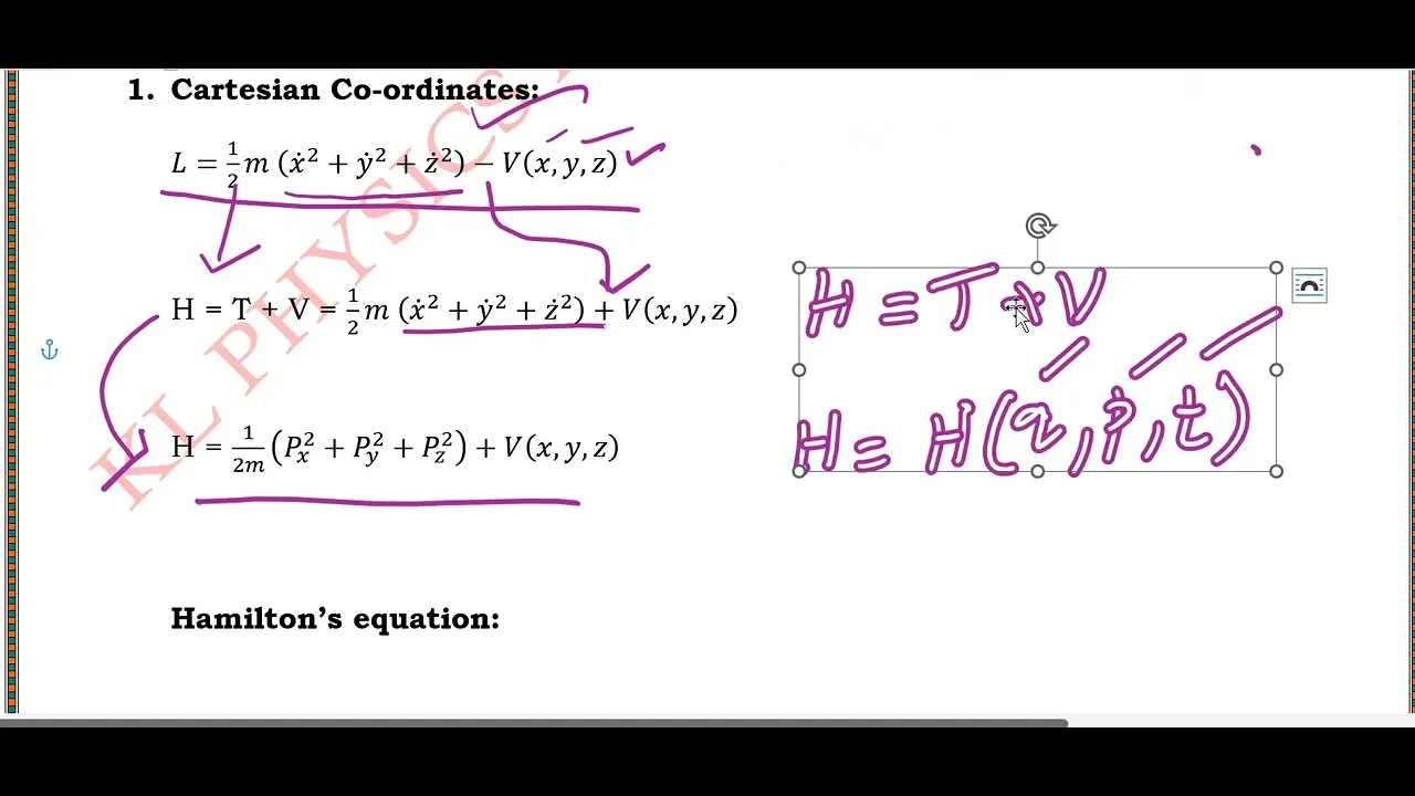
[00:00:18]So the example that we are going to use is the a particle that is in a uniform gravitational field. So we know that if the gravitational field is uniform the Hamiltonian that is going to correspond to this particle is going to be the next it will be h equ= px 2 + p y 2 all divided by 2m. In this case, we are considering the motion of the object in two dimensions because it will have a kinetic energy associated with the velocity in the x direction and in the y direction. Okay. And then a potential energy that corresponds to m g y.

[00:01:09]Okay. Perfect.

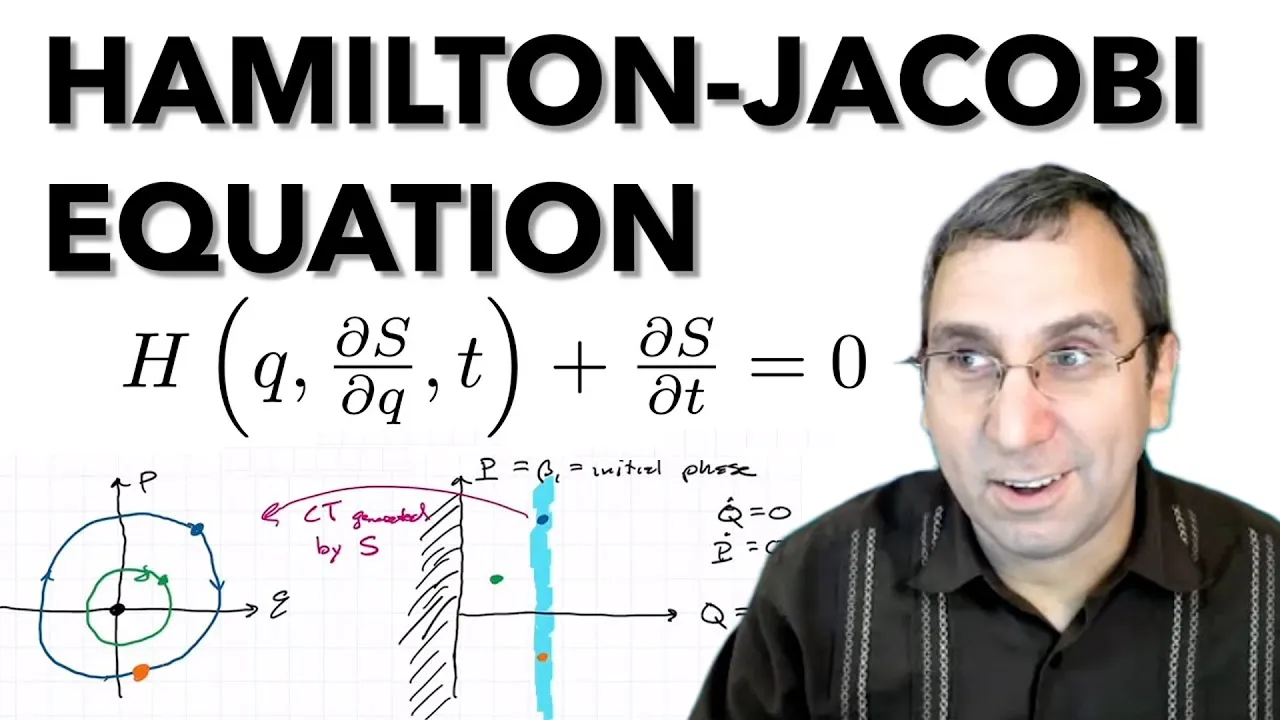
[00:01:12]of of course uh this mass is uh this m is the mass of the particle and g is the acceleration of gravity. So we remember that the Hamilton Hakovi equation says that a function h which is a function of in this case and we have two uh generalized coordinates Q which is going to be qx qy px py and the time and of course in our case we consider qx just as X and Q Y as Y. Okay, we have generalized coordinates for position and coordinates for the momentum that correspond to those generalized coordinates of position and then we sum the partial uh derivative of S with respect to time and this needs to be equal to zero.

[00:02:16]Perfect. So looking that we have two elements of um conjugate momentas we need to write them in terms of the partial derivative of this function s with respect to some generalized coordinates. Of course in this case uh we know that px is equal to the partial of s with respect to x and p y is equal to the partial of s with respect to y.

[00:02:42]So that means that the Hamington Hakobi equation takes the form h of x comma y comma the partial of s with respect to x the partial of s with respect to y the time plus the partial of s with respect to time equals to zero. So that will be the hamilton hakovi equation for a particle that is under a uniform gravitational field. And what happens if we take this Hamiltonian and uh we take the values of px and p y into it which correspond to the partials with respect to x and with respect to y. Well, we are going to get that we will have 1 / 2m that is going to multiply the partial of s with respect to x uh squar plus the partial of s with respect to y^2.

[00:03:39]Okay. So yeah and then plus mg y plus the partial of s with respect to time equals to zero. So this will be the Hamilton Hakobe equation for the particle in a uniform gravitational field. Perfect. Look that we have replaced the positions of px and py for the derivatives of s. Perfect. So the method that we are going to use consists in taking a function that is going to be of the variables x comma y comma t and express it as the sum of three functions of one variable. For example, a of x, b of y, and c of t. Look that these functions. Well, they are of just one variable.

[00:04:27]This a only depends on x and this b only depends on y. So, we are going to propose a solution for this equation given by this expression and we are going to see what happens. Well, of course, if we calculate the partial derivative of s with respect to x, looking that only a depends on x, we can set that this is equal to the derivative of a with respect to x, the total derivative because of course a only has one variable. So we can just take the total derivative and that will happen the same with the partial of x with respect to y. uh that will be equal to the total derivative of v with respect to y and the derivative of s with respect to time will be equal to the total derivative of c with respect to time. Perfect. So we can take this into the uh differential equation to get that 1 / 2 multiplies the derivative of a with respect to x^2 plus the derivative of b with respect to y^ 2 plus mg y equ= and let me take this into the right hand side of the equation to get minus the partial the sorry the derivative of c with respect to time.

[00:05:45]Perfect.

[00:05:47]And something that I want you to notice here that is very common when you use a separation of variables method in differential equations is to uh notice that the left expression on the equation is a function of some particular variables and the right hand side of the equation is a function of other variables. Yeah, this is very very common in solving differential equations that are partial differential equations.

[00:06:14]So we can say that this can be seen as a function of x and y while this is a function of t. So what happens if we have the derivative of a function of t in this side and then here we have a function of x and y which are different variables.

[00:06:39]Well, that means that well all this expression on the left hand side needs to be equal to a constant. And the same thing happens with with this uh element that we have here. It has to be equal to a constant because if we have a function of different variables that are equal, they can only be equal if they are constants. Okay? So if this thing over here is equal to a constant well we can set easily that c of t is going to be uh solution well it it will have the form minus p1 t where p1 is a constant. Okay, we have just uh encountered the solution for C taking the the well yeah we had that the derivative of C with respect to time is equal to a constant. If we take the integral then we get that this is equal to a linear function of t. Perfect. And actually uh you will have to notice in some further examples that this thing that we have here which is a linear function will occur very often if for example this t does not appear on the Hamiltonian. So what I'm saying is that looking that the t doesn't appear here in the Hamiltonian then this function c in the separation of variables uh proposal well is a linear function.

[00:08:10]Okay. So the t is not in the hamiltonian that means this c is a linear function.

[00:08:16]Perfect. Okay. So looking that this was equal to a constant then again the left hand side of the equation is also equal to a constant. So what is that what is that constant going to be? And well looking that we name this as p1. Of course, if we take the derivative of this, we get minus p1, but minus the derivative of that is just p1. So that means that we can set 1 / 2 m time the derivative of a with respect to x^ 2 plus the derivative of v with respect to y^ 2 + m y is equal to p1.

[00:08:56]Perfect.

[00:08:58]So what we are going to do next is to solve this equation for the derivative of a with respect to x. So we are going to get the derivative of a with respect to x² is going to be equal to it will be p1 minus mg y and then this multiplies 2 m minus the derivative of v with respect to y^2 and with the same um explanation that we gave before. This is only a function of x and this is only a function of y. So if we have two functions of different variables on both sides of the equation, that means that they need to be equal to a constant.

[00:09:52]Okay. So what we are going to set is that we will have that uh the derivative of a with respect to x^2 will be equal to well maybe p2.

[00:10:13]taking that the derivative of a with respect to x will be seen just as a constant p2 and making that a as a function of x will be equal to p2x.

[00:10:28]Perfect.

[00:10:29]Let me close this and also let me close the solution that we found for the c.

[00:10:38]Okay, perfect.

[00:10:41]So this takes us to get that well the derivative of a with respect to x is of course p2 and uh the derivative of a with respect to x^2 is um p2.

[00:10:55]Okay. So getting back to this equation we are going to get that p2 is equal to p1 and let me multiply by that 2m this 2 m p1 - 2 m^ 2 g y minus the derivative of v with respect to y² like this. So now we are interested in finding a solution for uh the derivative of v with respect to y. So if we work a little bit we are going to get that the derivative of v with respect to y can be seen as plus minus the square t of 2 m p1 minus p2 - 2 m^ 2 g y.

[00:11:50]So um yeah the thing here is that well we do not have to care about these two signs we can only choose one looking that we are looking for one solution. So there is no problem if we just take into account the positive solution. So if we remember uh the solution proposed was a + b + c. So that means and yeah let me establish that b is equal to well um the integral of the square root of 2 mp1 - p2 - 2 n^ 2 g y d y. So this takes us to establish the solution s = to well a a of x with that was a p 2x and then b of y which is this integral that we have here 2 m p1 - p2 2 - 2 m^ 2 g y d y and then plus c of t but that was equal to p1 t. Perfect. So now we have found a solution for the Hamilton Hakobe equation as uh the sum of three functions that are um of just one variable. Okay, perfect. Remember that on the first lesson that we have given in Hamilton Hakovi formalism, we established some equations that the the function needs to to verify.

[00:13:21]One of those equations is that um pi needs to be equal to the partial of s with respect to qi where this pi is the little p. Don't get confused. Remember we have little p and upper p. So uh the other equation was that uh the upper q is equal to the partial of s with respect to uh the upper p i. Okay, these are the equations that we showed on that first lesson. In this case, i goes from one up to two and they are equivalent to the x and the y.

[00:14:01]So that means that we are going to consider that here is going to be p x which is going to be the partial of s with respect to x and with these cues we are going to remain with the number notation. Okay. So that means that this will be Q1 = to the partial of S with respect to P1 and the other equations will be P Y = the partial of S with respect to Y and Q2 will be the partial of S with respect to P2.

[00:14:34]So with these equations and with the solution that we found we are able to find uh px, q1, py and q2. So px if we take the derivative of s with respect to x looking that this this element does not have an x and this element does not have an x that means that the partial of s with respect to x is only going to be this p2 that we have here. So the first result is going to be that px is equal to p2. Recall this is little p and this is upper p. Perfect. So what happens with for example PY?

[00:15:17]Well, PY is going to be equal to the and let me close this. PY is going to be the partial of X with respect to Y. So this one does not depend on Y. This one does not depend on Y. So we just need to take the partial derivative with respect to Y of this element that we have here. But looking that we are taking the derivative of an integral. Looking that they are inverse operators. Well, we are just going to make that uh we cancel the integral like if that is the correct way maybe. Um so that means that this py is going to be equal to what is inside the integral. So that's that means that we will have here the square<unk> of 2 mp1 - p2 - 2 m^2 g y. Perfect. So this will be the value of little p y. Okay. So what we are going to do now is to calculate what is q1. Well, we need to take the partial derivative with respect to p1 of this integral that we have here. So this will be equivalent to the yeah the integral of the partial derivative with respect to p1 of that square root that we have there which I'm going to write like this 2 m p1 minus p2 - 2 m^ 2 g y uh d y. Yeah, I just switch the order of the integral and the derivative because that is legal. Don't worry.

[00:16:59]So, and yeah, this is raised to the 1/2 power. So, let me take the derivative.

[00:17:05]This will be the integral of 12 2 m p1 - p2^ 2 - 2 m ^2 g y to the - 12 and then the derivative with respect to p1 of what is inside due to the chain rule which is just going to be 2 m.

[00:17:27]So this two cancels with this two. We got uh dy here. So that means that Q1 is going to be equal to the integral of M divided the square root 2 MP1 - P2 - 2 M^ 2 GY uh dy.

[00:17:50]Okay. And look here that well the function S that we found has a P1 here and a P1 here. So we still need to take the partial derivative with respect to p1 of this which is just going to be a t well a minus t actually. So that means that we need to add a minus t here a minus t here and a minus t over here.

[00:18:17]And I'm not going to solve this integral because well I think that is not necessary but I'm going to tell you what is the result if you make this integral remember it's just an integral uh of y it shouldn't be so hard but the result is that minus1 / mg the square root of 2 m p1 - p2 - 2 m^ G Y. So this will be Q1.

[00:18:52]Perfect.

[00:18:54]Okay, this is Q1.

[00:18:57]So we are going to calculate now Q2 which is the partial of S with respect to P2. So it will happen something very similar. Here we have a an element that depends on P2. So the partial uh with respect to p2 of this element is going to be x and then we need to take the partial of everything of this with respect to p2 is going to be very similar to the procedure that we just followed. So q2 is going to be equal to x plus the integral of the partial with respect to p2 of 2 m p1 - p2 - 2 m^ 2 g y raised to the 12 d y.

[00:19:47]So again we are going to calculate the derivative is x + the integral of 12 * 2 m p1 minus p2 - 2 m^ 2 g y to the -2 and then times the derivative with respect to p2 of what is inside.

[00:20:11]So that is - 2 p2 and then d y. Perfect.

[00:20:18]So we get x we cancel these twos plus the integral of p2 divided by the square t of 2 m p1 minus p2 - 2 m^ 2 g y and then dy here. Perfect. Again, we are not going to solve this integral. If we do that, the video will be very long.

[00:20:46]So, this is going to be equal to x + p2 here. That is going to divide m^ 2 g and it's going to multiply the square root of 2 m p1 - p2 - 2 m^ 2 g y.

[00:21:06]Perfect. This will be the result for q2.

[00:21:09]So um let me write you these four results u here in this page. These are the four equations that we just found.

[00:21:19]Remember that um before introducing the Hamilton hagobi formalism we were talking about some canonical transformations that they need to accomplish that they are functions of uh the generalized coordinates and the conjugate moments. Remember that if we find a canonical transformation that is equivalent to say that we have a new function Q and a new function P that are functions of the Q and the P and yeah only functions of Q and P that happens the same with the P. Okay. But in this case uh we have found uh these canonical transformations. But look here that for example this Q depends on the upper P uh the upper P1 and the upper P2 actually. So we do not want that. We would like to have a function Q1 that will be only a function of maybe Y and and maybe X and the time. Okay. but not a function of the upper P. So we need to solve these equations to get these kind of functions. You will see it in this example. So for example, let's look at this first equation that we have here.

[00:22:40]We can see that this P2 this upper P it is actually PX little px.

[00:22:50]So um with that we can solve this equation for P1 and in that case we will have a function P1 that will be only of the variables PX, PY and Y. So that is what we are actually looking for. So what are we going to do? Well, let me establish this as py 2 + p2 + 2 m 2 g y = to 2 m p1. Yeah. Okay. Yeah. And remember that this p2 is equal to px. So we get px². This is little p remember.

[00:23:34]So it is easy to see that p1 is going to be equal to 12 1 actually divided by 2 m* px 2 + p y^ 2 plus m g y okay because remember these two m will cancel these two m that we have here. So we only get an m on the numerator. Perfect. So we have found the first canonical transformation for the upper P1.

[00:24:09]Okay. So with this value that we just found, we can find this Q1 that we have here because we know what is P1. We know what is P2. So we are going to substitute those values into that expression. So we are going to get that q1 is equal to minus t minus 1 / mg the square<unk> of 2 m p1. But that p1 is going to be this that we just found which is 1 / 2 m px^ 2 p y^ 2 um + mg y like this.

[00:24:51]So that is 2 mp1 and then we will have minus p2 but p2 is px. So px^ 2 - 2 m^ 2 g y. Recall that for now um this function q1 is already a function of the generalized coordinates and the conjugate momentas little p and little q. So if we keep simplifying we will get minus t -1 / mg the square t of um px^ 2 p y^ 2 + 2 m^ 2 g y - px^ 2 - 2 m^ 2 g y and we can cancel this we can cancel this to get that q1 is equal to minus t -1 / mg g and the square root of py squar. And we are not we are not going to worry about the absolute value of the py. We're just going to take um one of the values that will be perfectly acceptable. So q1 will be minus t minus py divided by mg. Perfect. So with this we have found uh Q1 in terms of the little P and uh the variable T.

[00:26:20]Okay.

[00:26:22]Okay. And let me write in this step that P2 as a function of these little coordinates is equal to PX.

[00:26:35]So we are just need we are left with um the q q2 function. Okay. So that is this one over here. We have now the p2 we have the p1.

[00:26:51]So we need to substitute that into this expression to see what are we going to get. Let me rewrite this equation.

[00:26:58]Okay. So if we substitute the values that we have found we are going to get that Q2 is equal to X + P2 which is PX / M^ 2 G * the square t of 2 MP1 which is 1 / 2 M P 2 + P Y 2 + MGY I and then - px^ 2 which is p2 - 2 m^ 2 g y.

[00:27:38]Okay.

[00:27:40]So this is x + px / m^2 g.

[00:27:46]Here we will have px 2 + p y 2 + 2 m^ 2 g y - px^ 2 - 2 m ^2 g y. This cancels this cancels and we see easily that q2 is equal to x + px m^2 g again uh p y perfect. So that is the function Q in terms of the little variables. So with this we have now completed the transformation the canonical transformation that corresponds to uh the particle under the gravitational field that is uniform.

[00:28:34]So remember that we mentioned that the Hamington Hakobe equation comes from thinking that this canonical transformations lead us to a new Hamiltonian that is equal to zero. And that means that the derivatives with respect to time of these new functions that we found are equal to zero.

[00:29:00]meaning that these functions are constants. So if we are able to express the q well the x the y the px and the py in terms of these variables looking that they are constants well those functions those new functions will be equivalent to the solutions of the equations of motion of the mechanical system that we are studying. Okay, let's say for example that we are able to express this x as a function of q1, q2, p1, p2 and the time. Looking that these are all constants.

[00:29:43]Well, this means that we will have a function equivalent to x of t which is of course the solution of the motion of the particle that we want to find. So this means that we need to find the expressions for these four variables in terms of the upper variables. So how are we going to do that? Well, by now we already know that px is equal to p2.

[00:30:11]So this means that well this is already an equation of motion. It tells us that the momentum in the x direction is a constant because p2 is a constant.

[00:30:25]Okay, this is the first solution that we have. Perfect.

[00:30:30]We have uh found also that q1 is equal to minus t minus py / mg. So we can solve this easily for py.

[00:30:45]we will get that py / mg is equal to minus t + q1.

[00:30:52]So py is equal to minus t + q1 mg.

[00:31:00]Okay, perfect. So this means that this is another equation of motion that is telling us something about the momentum in the y direction. the momentum of the particle uh it well we see here that it is not a constant it depends on the time so it it changes on time and yep this can be seen as a function p y of t so this is the second solution so what happens with the x and the y well we found that uh the q2 that we have here is is this equation But uh we can set that this is q2 minus px p y / m^ 2 g is equal to the x.

[00:31:49]But we know that px is equal to p2.

[00:31:54]Yeah. And py is all this thing. So that means that x is equal to q2 minus p2 / m^ 2 g * py. But that is minus all this thing with this minus is going to be a plus. And then mg t + q1. So x is going to be q2 plus p2 / m * t + q1.

[00:32:30]Perfect. Again we have found x in terms of the time and some constants. So this is equivalent to say that this is the equation of motion uh in the x direction.

[00:32:43]Perfect. So we need to still find an equation for y.

[00:32:50]But remember we found that p1 is equal to p y ^2 + px^2 / 2 m + mg y. So from this we are going to solve for y and we get that what are we going to get? We get that p1 minus p y^2 + px 2 / 2 m is equal to mg y but p1 remains the same minus p y^ 2.

[00:33:25]What is p y^2?

[00:33:28]Well, it will be this thing squared.

[00:33:32]So, it will be equivalent to write the next t + q1 2 m^2 g 2 and then plus px² but px is p2. So P2 okay all this is divided by 2 M and this is equal to MG Y.

[00:33:59]So we will get that y is equal to p1 / mg minus okay with this my y dividing here we will only get a g surviving at the numerator.

[00:34:20]So this will be t + q1 g and these two in the denominator.

[00:34:29]and then minus p2 / 2 m^ 2 g and this term is squared of course. So yep I think this is the final result. We have found a function of y in terms of the time which is the solution of the particle in a uniform gravitational field. In this case uh remember the p1 and the p2 are constants. So this is equivalent to the equation of motion in the y direction.

[00:35:03]Okay, perfect. So this will be the four results that are important in this lesson.

Up Next

Geodesics: When Shortest Distance Isn't a Straight Line

@ParthGChannel

81.5K views•2021-06-01

Fluorescence & Jablonski Diagram | Molecular Photophysics

@yairmeiry

192.2K views•2012-01-12

NMR Spin Physics I: Zeeman Effect, Resonance Condition & Larmor Frequency

@nptel-indianinstituteofsci8064

2.3K views•2024-01-17

Entropy and the Second Law of Thermodynamics Explained

@veritasium

27.5M views•2023-07-01

Related Study Plans & Knowledge Roadmaps

Structured learning paths in Physics

View All Physics Topics

Analytical Mechanics: Lagrangian & Hamiltonian

01Mathematical Foundations: Calculus of Variations

02From Newtonian Mechanics to Constraint Dynamics

03The Principle of Least Action & Lagrangian Mechanics

+ 3 more learning modules

Explore Roadmap

General Relativity (Spacetime & Cosmology)

01Foundations of Relativity: Special Relativity

02The Geometry of Spacetime: Equivalence Principle & Curvature

03Einstein's Field Equations: The Mathematics of Gravity

+ 2 more learning modules

Explore Roadmap

Chaos Theory: Pendulums, Bifurcation & Limits

01Foundations of Classical Mechanics and Pendulums

02The Transition to Nonlinearity and the Double Pendulum

03Core Principles of Deterministic Chaos

+ 3 more learning modules

Explore Roadmap

Optics (Lenses, Wavefronts & Instruments)

01Foundations of Light and Geometrical Optics

02Mirrors, Lenses, and Image Formation

03Wave Optics: Wavefronts and Interference

+ 2 more learning modules

Explore Roadmap