Mastering Chaos Theory: Nonlinear Systems, Pendulums, and Predictability in Physics
Learning Goals: Develop a deep, rigorous understanding of classical mechanics' transition into deterministic chaos. Learners will master the physics of linear vs. nonlinear systems, qualitative and quantitative tools for analyzing chaotic systems (including phase space portraits and Lyapunov exponents), the geometric properties of fractals and strange attractors, period-doubling routes to chaos, and the fundamental limits of physical predictability exemplified by the Three-Body Problem and weather dynamics.
- Estimated Total Study Time: 18 hours
- Prerequisites: Basic classical mechanics (kinematics, Newton's Laws), introductory calculus (derivatives and basic differential equations).
Module 1: Foundations of Classical Mechanics and Pendulums
This module establishes the baseline transition from simple, predictable systems to nonlinear classical mechanics. You will review Simple Harmonic Motion (SHM) using a simple pendulum and learn to differentiate linear and nonlinear ordinary differential equations (ODEs). Finally, you will learn how to graphically represent system state trajectories using qualitative Phase Space portraits.
Recommended Videos
Why this video: This video provides the essential physical setup of a simple gravity pendulum. It explains the mechanics of the restoring force and demonstrates how the pendulum serves as the standard introduction to periodic, simple harmonic oscillations when analyzed in ideal, non-dissipative environments.

Why this video: To understand why chaos only occurs in nonlinear systems, you must mathematically distinguish linear ODEs from nonlinear ones. This tutorial breaks down the formal definition of linearity in differential equations, focusing on the powers of the dependent variables and their derivatives.
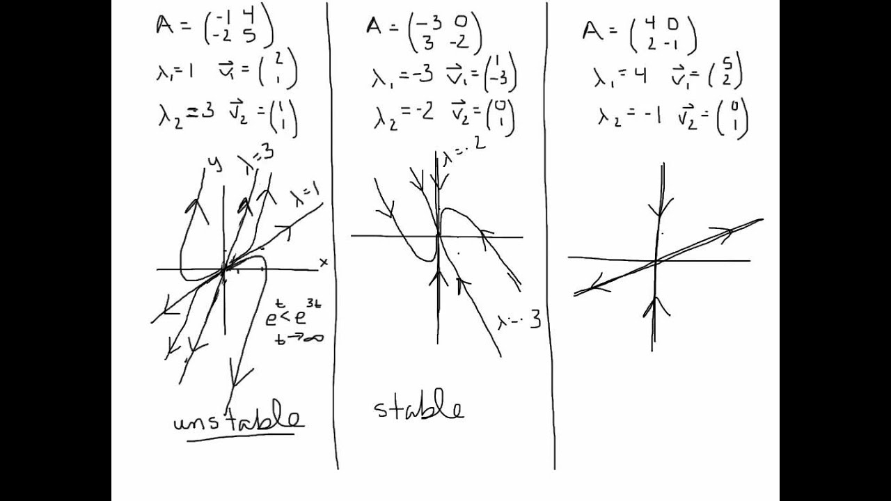
Why this video: Phase space is the core visualization framework for dynamical systems. This comprehensive lecture walks you through the step-by-step process of plotting phase portraits for differential equations based on eigenvalue classifications (stable/unstable nodes, saddles, and centers). This qualitative mapping is vital for analyzing systems where closed-form analytical solutions do not exist.
Knowledge Checkpoint
- Understand how the small-angle approximation () linearizes the pendulum's equation of motion.
- Classify a given ordinary differential equation as either linear or nonlinear based on the exponents and coefficients of the dependent variables.
- Identify and sketch fixed points, trajectories, and vector directions in a 2D phase portrait for stable nodes, unstable nodes, and saddle points.
Module 2: The Transition to Nonlinearity and the Double Pendulum
Building on Module 1, you will investigate what happens when a classical system gains a second degree of freedom. By coupling two simple pendulums, the system transitions from predictable harmonic motion to chaotic dynamics. This module introduces Lagrangian mechanics and demonstrates how slight variations in initial conditions completely change the resulting complex trajectories.
Recommended Videos
Why this video: This clip visually demonstrates how a simple mechanical system—the double pendulum—exhibits three distinct behaviors depending on its energy state: low-amplitude periodic motion, out-of-phase periodic motion, and complex, unpredictable chaotic motion. It connects physical execution directly to Newton's underlying laws.

Why this video: To truly understand the chaotic dynamics of a double pendulum, you must examine its equations of motion. This video walks through the physics equations derived from Lagrangian mechanics and demonstrates how to implement a numerical solver to simulate the double pendulum's motion, highlighting its extreme sensitivity to starting values.

Why this video: This classic lecture excerpt explains nonlinear autonomous systems. It lays out the formal mathematical foundation for systems of first-order differential equations containing quadratic or trigonometric terms, helping you bridge the physical behavior of double pendulums with rigorous differential math.
Knowledge Checkpoint
- Explain how a double pendulum's behavior shifts from predictable periodic motion at low energy levels to chaotic motion at high energy levels.
- Explain why the Lagrangian framework is preferred over Newtonian force vectors when deriving equations of motion for multi-degree-of-freedom systems.
- Identify a "nonlinear autonomous system" and explain why its state derivatives depend only on the state variables themselves, rather than explicit time variables.
Module 3: Core Principles of Deterministic Chaos & Lyapunov Exponents
This module addresses the central paradox of chaos theory: how systems governed by strict, deterministic equations of motion can become completely unpredictable. You will explore the "Butterfly Effect" (sensitivity to initial conditions) and learn how to quantitatively measure chaotic divergence using Lyapunov Exponents.
Recommended Videos

Why this video: This highly visual explainer highlights the discovery of chaos in the Lorenz equations. It shows how starting multiple trajectories with nearly identical coordinates leads to divergent pathways in state space, introducing the conceptual foundation of the Butterfly Effect.
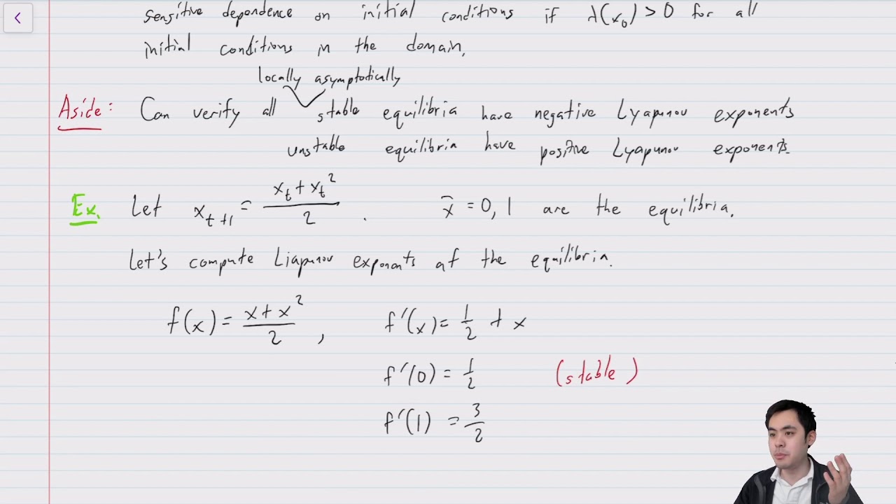
Why this video: This mathematical lecture defines the Lyapunov exponent ()—the key quantitative metric of chaos. It explains how to measure the average exponential rate of divergence between two infinitesimally close trajectories.
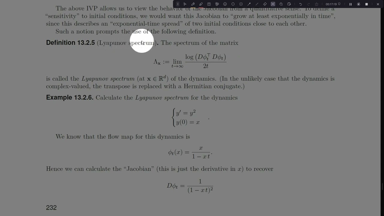
Why this video: A rigorous, long-form academic lecture that connects the physical principle of sensitivity to initial conditions with its strict mathematical definitions. It provides a formal framework for calculating Lyapunov exponents in continuous dynamical systems.

Why this video: This video focuses on discrete maps (such as the logistic map). It details the mathematical formula used to calculate the Lyapunov exponent (), showing how a positive exponent () serves as a mathematical proof of chaotic behavior.
Knowledge Checkpoint
- Define "determinism" and explain how a system can be entirely deterministic yet practically unpredictable.
- Mathematically define the Lyapunov exponent () and interpret the physical significance of , , and .
- Calculate the Lyapunov exponent for a simple 1D discrete map given its derivative equation.
Module 4: Strange Attractors and Phase Space Geometry
In this module, you will master the geometric structures that organize chaotic systems. While linear systems settle into points or limit cycles, chaotic systems converge onto infinitely complex, self-similar geometric objects known as Strange Attractors. You will explore the 3D phase space geometry of the Lorenz Attractor and examine the fractured dimensions of fractals.
Recommended Videos
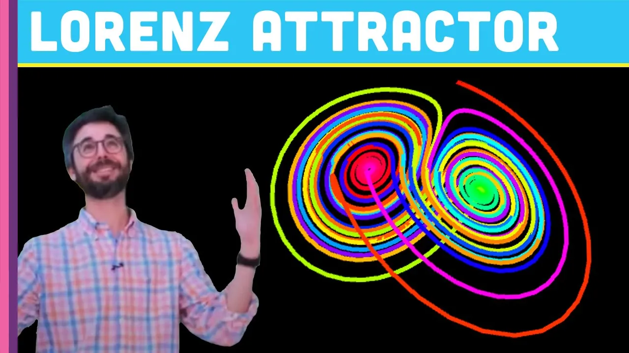
Why this video: This coding walkthrough details the differential equations that define the Lorenz system (, , ). By simulating these equations in 3D, you will see how chaotic trajectories trace out the famous butterfly-shaped strange attractor.

Why this video: This video introduces fractals—objects characterized by self-similarity and non-integer ("fractured") spatial dimensions. It provides intuitive physical examples from nature (rivers, lightning, blood vessels) to explain the concept of fractional dimension.

Why this video: This deep dive connects the geometry of strange attractors to physical states. It shows how the boundaries between different basins of attraction in multi-stable physical systems have fractal geometries, making it impossible to predict which stable state the system will select.
Knowledge Checkpoint
- Write out the system of three ordinary differential equations that define the Lorenz Attractor.
- Explain what makes an attractor "strange" compared to a classic point attractor or limit cycle.
- Explain the concept of fractal dimension and how it relates to phase space trajectories that never intersect themselves.
Module 5: Bifurcations and the Route to Chaos
This module analyzes how ordered, predictable systems transition into chaos. Using the Logistic Map () as a model, you will study how changing a single control parameter () forces the system through period-doubling bifurcations, culminating in chaotic dynamics governed by the universal Feigenbaum Constants.
Recommended Videos
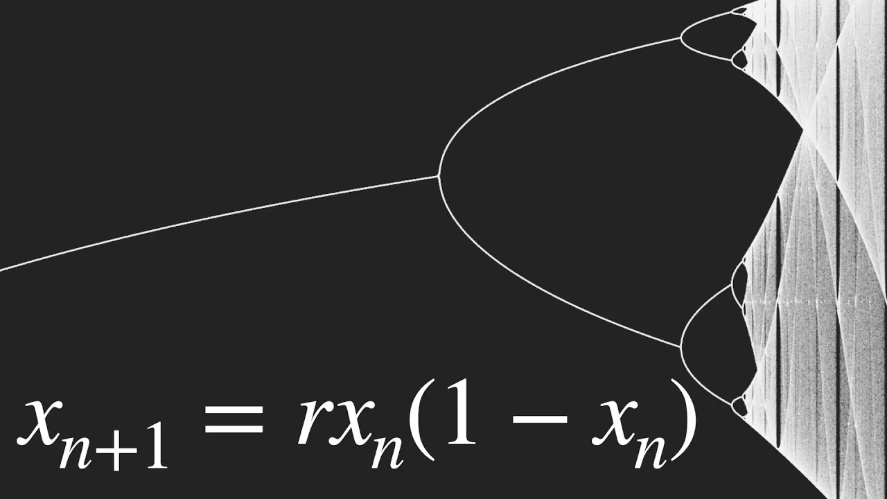
Why this video: This highly engaging video traces the transition of the logistic map from stable single-value outcomes to period-doubling oscillations, and finally into total chaos at . It also highlights the spontaneous emergence of stable periodic windows within chaotic regimes.
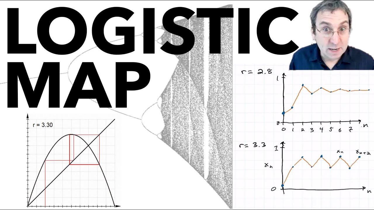
Why this video: This tutorial focuses on the mathematics of period-doubling. It explains how the ratio of successive bifurcation intervals converges to the first Feigenbaum constant (), demonstrating a universal pattern shared by many nonlinear systems.

Why this video: This lecture demonstrates how to construct and read a bifurcation diagram. It shows how fixed points () are plotted against a control parameter (), teaching you how to distinguish stable fixed points (solid curves) from unstable ones (dashed curves).
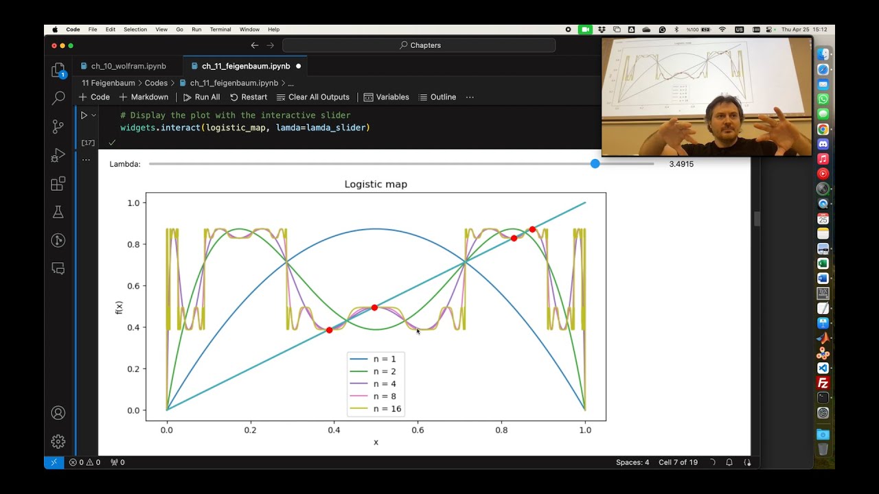
Why this video: This advanced lecture provides a technical explanation of the second Feigenbaum constant (). It uses renormalization theory to explain scaling behaviors near the threshold of chaos, connecting the bifurcation geometry of discrete maps with physical phase transitions.
Knowledge Checkpoint
- Write down the equation for the Logistic Map and identify the role of the growth/control parameter ().
- Describe the geometric structure of a bifurcation diagram and point out where period-doubling occurs.
- State the value of the first Feigenbaum constant () and explain its universal significance in nonlinear systems.
- Describe what happens within the "periodic windows" that emerge inside the chaotic regions of a bifurcation diagram.
Module 6: Predictability Limits and Real-World Applications
This final module applies chaos theory to real-world systems. You will study how deterministic chaos sets absolute limits on long-term predictions, focusing on two classic systems: weather forecasting and the planetary gravitational physics of the Three-Body Problem.
Recommended Videos

Why this video: This video introduces the Three-Body Problem—a fundamental challenge in celestial mechanics. While two-body systems (like a single planet orbiting a star) are stable and solvable, adding a third body of comparable mass creates a chaotic system that is highly sensitive to initial states and often results in orbital ejections.

Why this video: A detailed look at the mathematics and history of the Three-Body Problem, starting with Newton's initial attempts to solve it. It explains why no general closed-form algebraic formula exists to predict three-body motion, demonstrating how early physics encountered the limits of predictability.

Why this video: This video focuses on meteorological systems. It explains why weather forecasting is fundamentally limited by chaos theory, tracing back to Edward Lorenz's 1961 computer model where rounding variables by just three decimal places completely altered long-term simulation results.

Why this video: This advanced lecture from Oxford Mathematics clarifies common misconceptions about the butterfly effect. It focuses on finite predictability horizons in multi-scale physical systems, explaining why increasing the precision of initial measurements cannot extend predictions beyond a certain time horizon.
Knowledge Checkpoint
- Explain why two-body gravitational systems are integrable and solvable, whereas three-body systems are chaotic and have no general closed-form analytical solution.
- Define the term "predictability horizon" and explain how it limits weather forecasting models despite advances in supercomputing.
- Contrast a simple chaotic system with a complex, multiscale chaotic system (like the global atmosphere) in terms of predictive limits.
Course Map
This flowchart outlines the recommended pathway through the curriculum, highlighting the dependencies between the conceptual models.
Key People Index
| Practitioner | Historical Context & Contribution |
|---|---|
| Sir Isaac Newton | Formulated classical laws of gravitation; solved the two-body problem but hit a wall trying to resolve the three-body Earth-Moon-Sun system. |
| Henri Poincaré | Often cited as the true father of chaos theory; discovered deterministic chaos while entering a contest to solve the Three-Body Problem in the late 19th century. |
| Edward Lorenz | American meteorologist who discovered the "Butterfly Effect" in 1961 while simulating atmospheric currents; defined the simplified Lorenz system of equations. |
| Aleksandr Lyapunov | Russian mathematician who developed the quantitative metric (Lyapunov exponent) used to measure the exponential divergence rates of nearby trajectories. |
| Robert May | Australian ecologist whose 1976 paper on the discrete logistic map popularized the period-doubling route to chaos in population dynamics. |
| Mitchell Feigenbaum | American physicist who discovered universal constants ( and ) that describe how fast period-doublings scale in nonlinear maps. |
| Benoit Mandelbrot | Polish-born mathematician who coined the term "fractal" and defined the mathematics of fractional scaling dimensions. |
Final Self-Assessment
Complete this checklist to verify your mastery of Chaos Theory.
- Linearity vs. Nonlinearity: I can mathematically identify a nonlinear differential equation and explain why nonlinearity is a requirement for chaotic dynamics.
- Small-Angle Limits: I can derive the equation of motion for a simple pendulum and explain how the small-angle approximation linearizes the system.
- Phase Space Sketching: I can qualitatively map out trajectories, fixed points, and vector directions in a 2D phase portrait from any autonomous 2D system of linear ODEs.
- Double Pendulum Physics: I can explain why the double pendulum has two degrees of freedom and how its phase space transitions from closed periodic orbits to chaotic trajectories as total system energy increases.
- Quantitative Chaos: I can write out the analytical definition of the Lyapunov Exponent () and prove how a positive value () implies chaos.
- Lorenz Attractor Equations: I can write down the three Lorenz equations and describe the physical weather-modeling approximations that inspired them.
- Strange Attractor Geometry: I can explain why trajectories on a strange attractor in a finite phase space can never intersect themselves or repeat exactly.
- Logistic Map Bifurcations: I can draw a bifurcation diagram of the logistic map and label the stable points, the period-doubling points, and the chaotic regime.
- Feigenbaum Universality: I can define the first Feigenbaum constant () and explain why it applies to systems beyond the logistic map.
- The Three-Body Problem: I can describe the physical mechanism of chaotic instability in three-body systems and explain why no general algebraic solution exists.
- Limits of Predictability: I can explain why infinite computing power and highly precise measurements cannot yield infinite-horizon weather predictions.