




![Математические методы классической механики В. И. Арнольда [1] // Николай Тюрин](https://i.ytimg.com/vi/VIZ7OP4WNbQ/hqdefault.jpg)



![839 - CALCULUS (TempleOS | Livestream) [2016]](https://i.ytimg.com/vi/qBuMzDpnkRM/sddefault.jpg)









![Estabilidad por LYAPUNOV 📕 [Sistemas Dinámicos Lineales] #012](https://i.ytimg.com/vi/77u0OC96mec/sddefault.jpg)
Phase portraits for linear constant coefficient systems of differential equations are classified by eigenvalue types: for real eigenvalues, positive values create unstable nodes (solutions diverge from origin), negative values create stable nodes (solutions converge to origin), and mixed signs create saddle points; for repeated eigenvalues, the direction is determined by testing a point; for complex eigenvalues, the real part determines stability (negative = stable spiral, positive = unstable spiral, zero = center) while the imaginary part indicates oscillation, with direction determined by matrix multiplication with a test point.
Sketching Phase Portraits for Linear Systems of Differential Equations
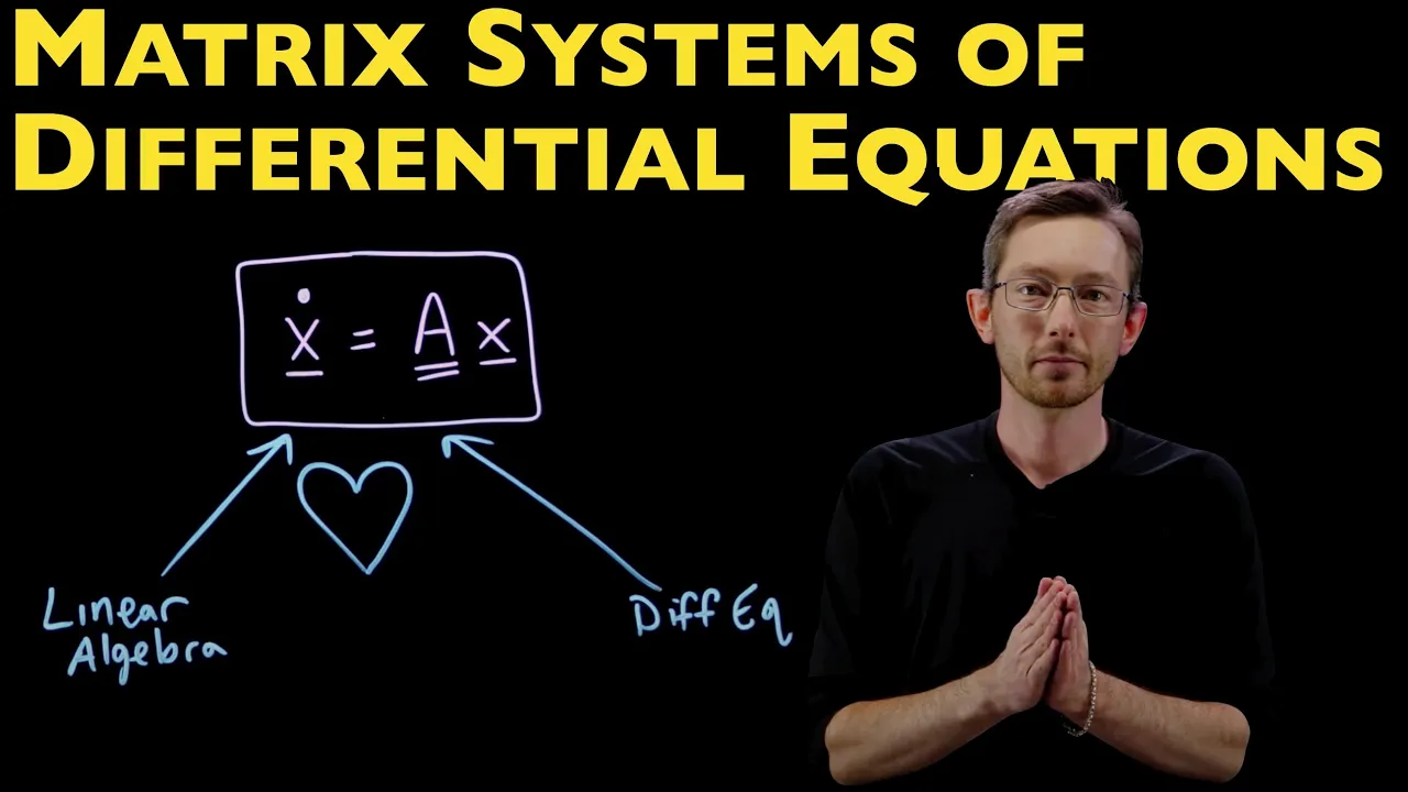
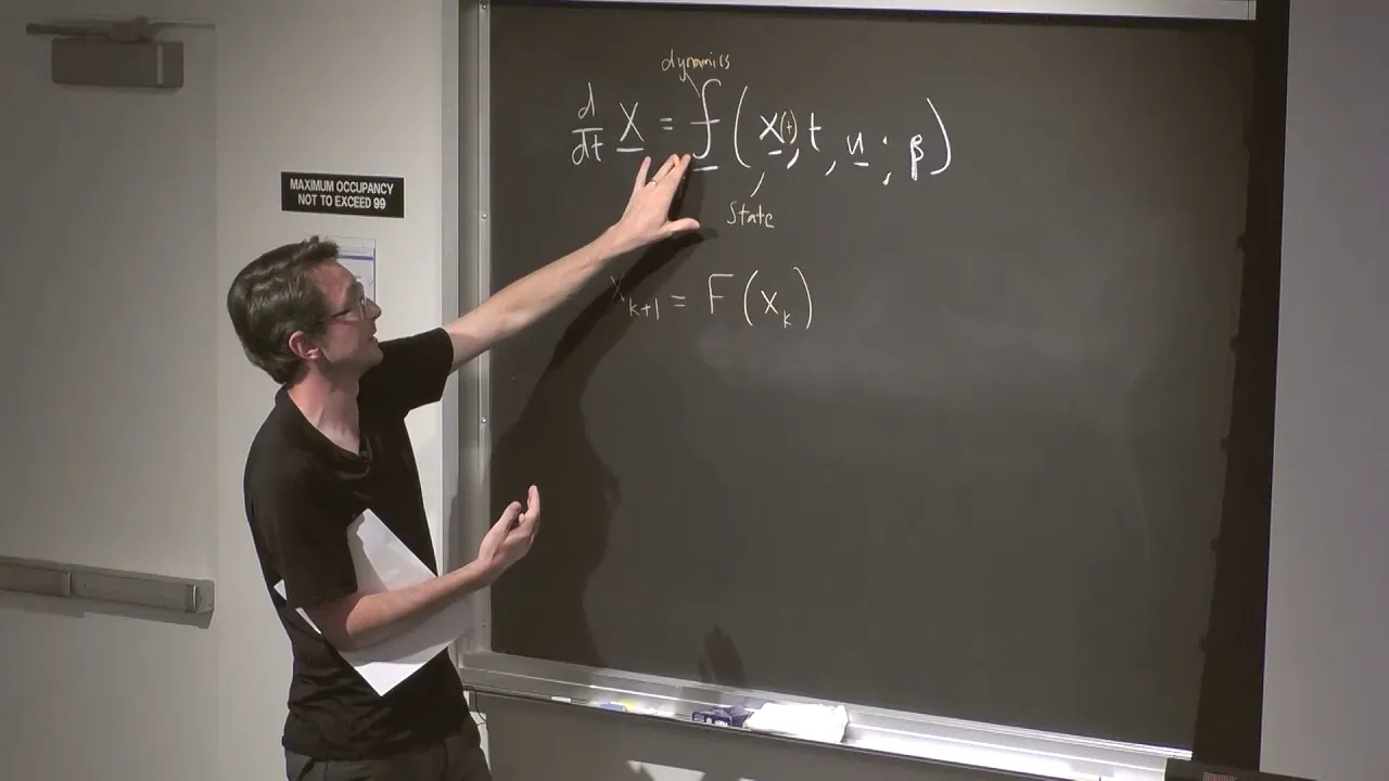
Added:Understanding the matrix representation of systems of first-order linear differential equations (dx/dt = Ax).
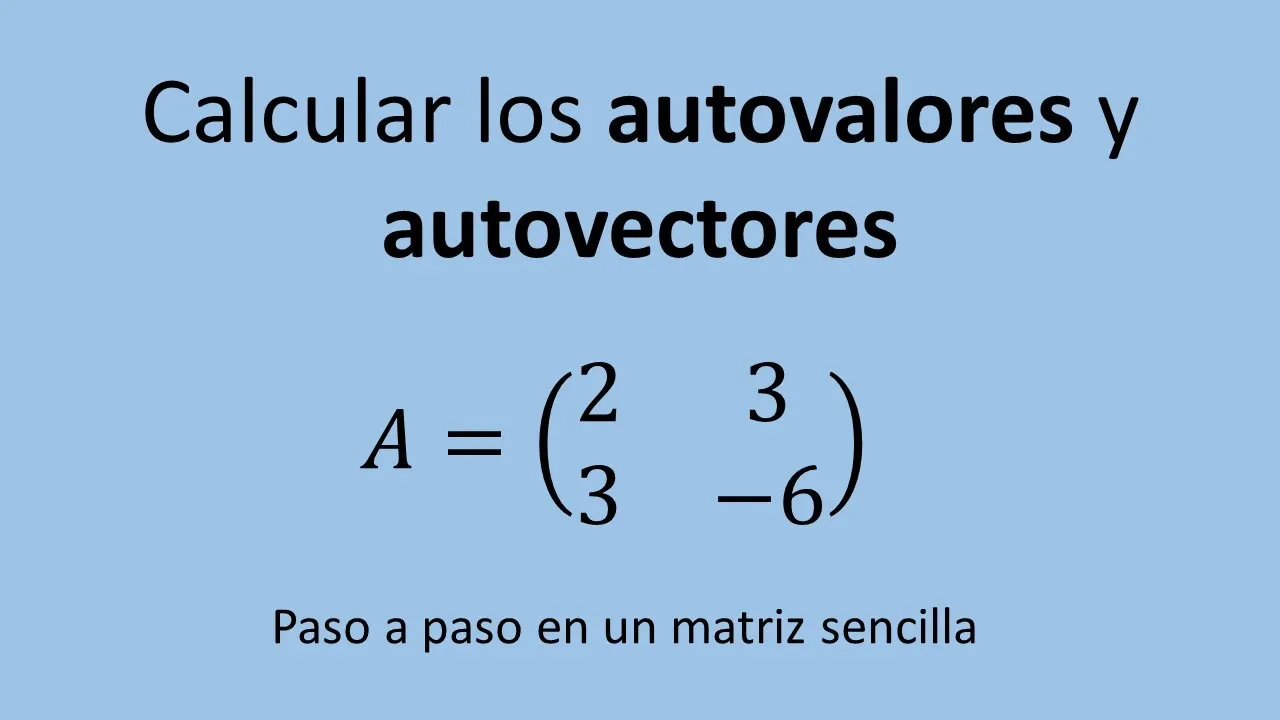
Proficiency in linear algebra, specifically calculating eigenvalues and eigenvectors of 2x2 matrices.
Familiarity with complex numbers and Euler's formula, which are essential for interpreting complex eigenvalues.
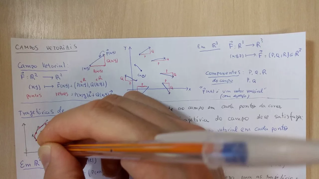
The basic concept of a vector field and how geometric trajectories represent solutions over time.
Linearization of nonlinear dynamical systems near critical points using the Jacobian matrix.
Exploring bifurcation theory to understand how phase portraits qualitatively change as system parameters vary.
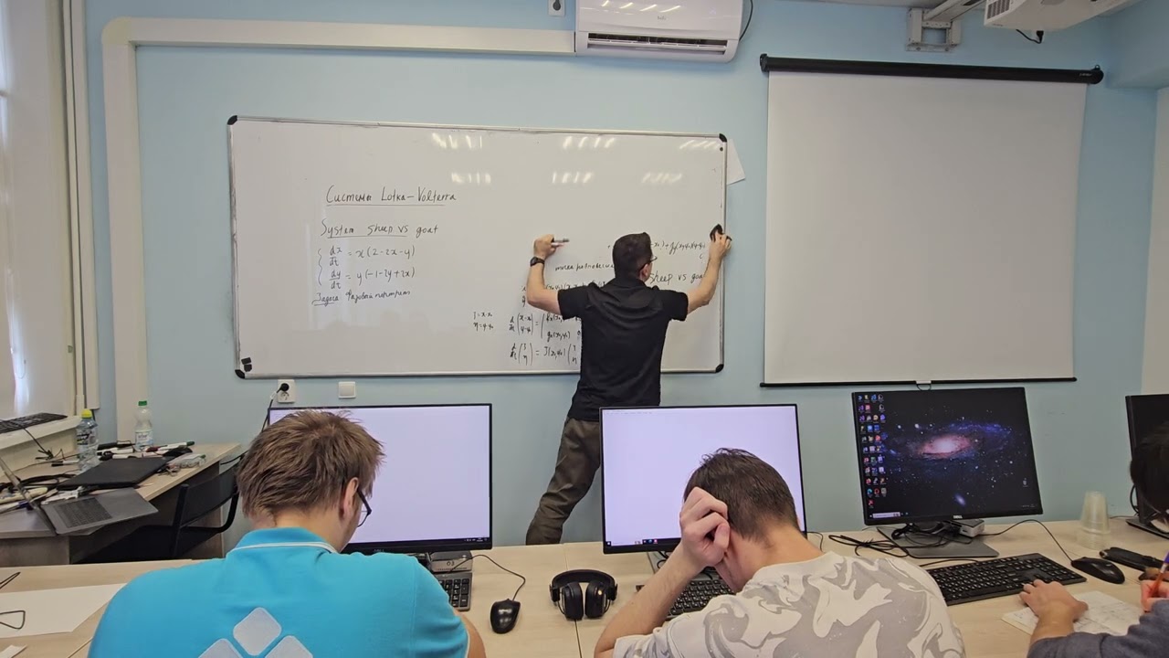
Applying phase portrait analysis to real-world models, such as the Lotka-Volterra predator-prey equations or coupled harmonic oscillators.
Studying rigorous stability analysis using Lyapunov functions for both linear and nonlinear systems.
542.8K views10.2Klikes20:00Original Release: 2015-03-12
all right this video is going to go over graphing phase portraits for linear constant coefficient systems of differential equations now the system of differential equation has an X and A Y component to it in a vector form so when we draw the phase portrait for it the phase portrait is going to be usually X on the um on the horizontal axis y on the vertical kind of like normal but what's different about these is that for each different solution trajectory so for the solution curve we're going to have an arrow and that represents the time variable involved in all of this there's lots of different graphs um it basically breaks down into three different ways to graph and they're different depending on whether there are two real igen values a repeated IG value or complex IG value and then those different parts depend on whether the igen values are well for the two real if they're both negative we get a different kind of a graph from if they're both positive um versus if one is negative and one is positive for the repeated igen value we're only going to look at what happens when they're positive and negative um it's called doubly degenerate when they are both zero um and we're not going to look at that case uh complex igen values um for these we only need to look at the real part since that's what what the exponential is raised to and that will tell us um stuff about the the system and we'll get there in just a second um but that's dependent on whether it's positive negative or zero just the real part the complex part also tells us that spy rolles because it oscillates um but the real part gives us a lot more information about the graph okay here we go so let's do the real IG values first all right here are three different matrices that would be associated with uh a system of differential equations there igen values for each one and Ian vectors for each one so you'll probably have to pause this video each different time we go through these um just so that you can write down the Matrix and its Associated IG values and igen vectors um so this is the information it's basic information we need actually all we need is the IG values and IG vectors to graph each one of those each one of these things so notice this is the case where they're all real igen values um on this first one here that's an equals not a negative both of those igen values are positive on the second one both igen values are negative and on the third one there's one positive and one negative and you'll see how this will affect each different system okay so for the first one and what we're going to do for every single one one of these is look at the igen vector and graph a vector that goes in the direction of that IG Vector okay so it goes 2 in the X and one in the Y so for X and Y that IG Vector goes 2 in the X 1 in the Y so there's a point I just went from 0 0 to 21 and I'm going to draw a line through that point in both directions and so that is a vector in the direction of 21 now because the igen value is positive that means all Solutions on this line would Trend away from the origin and I need to write down that Lambda is equal to 1 I need that for later so I graphed the igen vector put arrows on it to show that all solutions go away from the origin and that's because l that's because one is positive right here this one is positive um and then I marked it with which I value it was I'm going to do the same thing for that IG value of three the IG Vector is 1 one so there's a DOT at 1 one and I'm going to draw a line wow this is hard on this on this thing that goes through the origin it does just pretend this is hard to graph these okay so there's that line um sorry I'm going to back up and see if will it actually back up it won't can I erase because that looks horrible okay I'm going to try again see if I can actually draw a line on this thing all right just through one one okay better at least through the origin this time all right so now that one had a positive IG value again so positive arrows going away from the origin there they are going away and that one goes with Lambda equal 3 okay now all arrows are pointing away from the origin and what this means is that all solutions are going to point away from the origin so I'm going to start and I'm going to start right here near the origin and I know that as time goes to Infinity e to the 3 is going to be way bigger so here's my thought process is that e to the 3 T is going to be way bigger than e to the T as time goes to infinity and what that means is that all solutions are going to look like this IG value as time goes to Infinity which means that they're starting out looking like the other one so I'm going to start at the small Igan value or IG vector and Trend towards the big so notice I made it look parallel to the big one so now I'm going to come over to this region I'm going to draw another solution that's sort of representative in there but I need to start being parallel to the small one so I'm trying to figure out which one is the small one here that's that one and then it's going to become parallel to the big one as time goes to Infinity now just like before when Solutions went away from an equilibrium point it was called uh unstable it's the same here so this would be classified as unstable all right um I'm not going to draw solutions in this portion and this portion well let me just draw one and you can see why I wouldn't in general because they they sort of look funny so if I start being parallel to one and then become parallel to three you can sort of see it just looks a little bit strange guess I'll draw it in there just you can yeah it looks a little bit strange so depending on how close I vectors are together um I might not draw solutions in between them if they're too close Okay on to the next one same exact process um now this one has negative igen values which means that instead of arrows going away from they're going to go into so for the first one the I Vector was 1 -3 so I'm going to go to one 1 2 3 about there and attempt to draw a line through the origin and through that point okay and that one was associated with -3 and it's negative so arrows go in the next Dion Vector is 0 1 that means I go nothing in the X and up one in the Y and then draw a line through that in the origin so really this is just the Y AIS and again I value is negative so Solutions go in and that one was associated with y = -2 now the rest of the solutions are different the one on the left I started at the origin because all solutions sort of start at the origin and work their way out now on this one all solutions end at the origin so I need to start away from the origin and then work in and I need to start away from the origin parallel to the smaller igen value and then get close to the big one so let's see the smaller one is -3 so I'm going to start away from the origin and parallel to -3 like that away from the origin parallel to -3 and then I'm going to become parallel to the big one as this mors into the origin all right same thing kind of over here on the left I've got to figure out which one is -3 go parallel to that one and then as it comes into the origin it's going to swoop parallel to the one that was -2 all right and again I'm not going to draw them in between those two um because they're so close together um it doesn't it it makes it look just a little silly now this one all solutions go into the origin so this one is called stable all right next one vector is 52 so I'm going to go over five up two and draw a line there we go parallel to or through 52 now that one went with a positive IG value of four so Solutions go away because that's positive and then the next one was 0 1 so 0 in the X one in the y That's again the Y AIS and on that one Solutions are negative so arrows go in and that's because the igen value was negative of Nega 1 now this is called a saddle [Music] saddle um and these are a little bit easier to draw because you don't have to think about which one's bigger and smaller you can follow the arrow because the solutions do not tend towards nor away from the origin they do neither so I sort of I just follow the direction of the arrows so up here on the left I've got Arrow going down arrow going left so Solutions in that portion of it are going to go down and left upper right Solutions go down and right so down and right lower right Solutions go up and right and lower left Solutions go up and left so that's what a saddle would look like oops all right so here are two different systems with a single real igen value so repeated igen values now the Sim the process of graphing these starts out very similar where you look at the igen vector so in this first one the vector is 31 and then you draw a line 31 and draw a line sort of through 31 the I value is positive so all solutions tend away from the origin and now the trick is we don't know which way the solutions uh go from here because if you look up above that line Solutions are going to start at the origin and work their way out because everything's going away because of that positive I value and they're either going to Trend clockwise or counterclockwise now the way that I do this is I'm just going to pick a random point now I like the 1 that's like right over here on the x axis so I I just it's a nice point to pick now if I multiply that by a then what I get get is a vector so that would be the vector 2 * 1 is 2 + 0 is 2 and two or 1 * a 3 is a3+ 0 so that's a thir and so I get a vector and so from the0 1 Z this tells me that a vector goes in the direction 2 A3 so there's like a little tiny Arrow going in that direction from one zer so wow that is really hard to tell I don't like that Arrow I can't tell whether these are going clockwise or counterclockwise from it I'm going to pick a new Point 2 -3 1/3 4 let's try 01 another one that I like just cuz the zeros make it pretty easy so that would be a vector that would be in the direction of -3 and 4 so I'm going to go to 01 that's up here go in the direction of3 in the X pos4 in the Y so that's up that way okay so these that arrow is a little bit better and what it tells me is that Solutions are going to become parallel to that left hand Arrow um or kind of look sort of like it so I'm going to go then it also tells me that these go let's see which direction is that that is counterclockwise so counterclockwise there and kind of see how my arrow matches up there so Solutions in the other direction go the opposite way so once I've got one of these I can fill in the other by going the opposite direction okay let's look at this next one um by the way these are all going out again so that would be unstable and so in this other one vector is 1 2 so there's a line that's approximately one one over in the X and two up in the Y now everything is negative on this one that's because of that5 I need direction so I'm going to take a and multiply it by let's go for the one zero see if that works out for us that's a three right there uh so 1 Z would give us -7 -4 so if I go to 1 Z that's -7 in the X let say7 in the x -4 in the Y and solutions need to Trend towards the origin so in order to follow that Arrow they would have to start here go through that arrow and then become parallel to the other one and that means that Solutions are going to do the opposite on the other side and again Trend towards the origin and this one because they all tend Trend into the origin this one is called stable all right oops okay so now the complex igen values uh notice there's three different scenarios one where the real part is negative one where the real part is positive and one where the real part is zero and this is the part of the igen value so all that's needed on these is the igen value you don't need the igen vector because you get cosine and S these actually spiral so you get circular patterns with this now the -2 here says that we're going to go into the origin so just like the negatives before this would be stable but it's going to spiral and so we know it's going to go into the origin but we need to figure whether it does that clockwise or counterclockwise and the way to figure that out is to do the exact same thing we did with the real ones which is to take the the uh Matrix multiply it by a random point I like one0 so when you multiply this you get -2 + 0 0 and -3 plus 0 0 so then I go to the point 1 0 and then I graph an arrow approximately in the direction of -2 -3 and so if I follow that arrow that leads me clockwise so I know that these Solutions are going to go clockwise and into the origin like that so there's just one and I'm draw a couple arrows pointing into the origin I could draw more than one but one is sufficient all right on this next one notice that the igen value is positive all solutions are going to go away from the origin and we've been calling away from the origin unstable and specify that this is a little bit different than the other ones we're going to say it's an unstable spiral and again I need direction so I'm going to take that Matrix multiply it by one Z my favorite point and get 2 -3 so I go to the point 1 Z draw an arrow in the direction of 2 -3 and if I keep following that Arrow that is also going to be going clockwise and so I can draw a solution that's going to start at the origin and go clockwise and Away did I get arrows pointing away yes from the origin okay the next one there is a zero here which means that uh Solutions do not go into or away from the origin and so this is uh this is called a center sorry I was just about to write a spiral but it is called a center when Solutions go neither into nor away from the origin so these looks like circles or ovals I'm not going to get into the details of the circles or ovals those kind of more have to do with the with the Matrix itself um and these these vectors uh so all I need to figure out is Direction on this one I'm going to take that Matrix [Music] a multiply it by my favorite 010 and get 0 -5 so from the 0 1 0 I'm going to go 0 in the X and -5 in the Y so that would just point straight down and so that tells me once again clockwise it is possible these go counterclockwise I I picked um I picked three that went clockwise uh not on purpose okay so that would go clockwise like that so there's one solution um and again one on these is very sufficient to show exactly what would happen with all different types of solutions any solution trajectory
Up Next
57:40
Can Mathematics Predict the Future? The Limits of Chaos Theory
@GreshamCollege
24.6K views•2018-10-15

4:43
Elliptic Curve Cryptography Explained: ECC, ECDSA, ECDH
@PracticalNetworking
28.5K views•2024-10-21

10:44
Fourier Series Introduction: The Big Idea Explained
@DrTrefor
387K views•2021-05-03

6:00
The Mathematical Impossibility of Accurate World Maps
@Vox
23.3M views•2016-12-02
Related Study Plans & Knowledge Roadmaps
Structured learning paths in Mathematics
mathematics
Tensor Calculus: Vectors to Riemann Curvature
01Mathematical Foundations: Linear Algebra & Calculus
02Covectors, Dual Spaces, and Tensor Basics
03The Metric Tensor and Index Gymnastics
+ 2 more learning modules
40h5 modules
Explore Roadmap
mathematics
Gödel's Incompleteness: Logic, Proofs & Limits
01Introduction to Formal Systems & Hilbert's Dream
02Set Theory, Cardinality, and Cantor's Diagonal Argument
03Arithmetization and Gödel Numbering
+ 2 more learning modules
14h5 modules
Explore Roadmap
mathematics
Galois Theory: Fields, Groups & Solvability
01Foundations of Abstract Algebra: Groups & Fields
02Polynomials & Field Extensions
03Splitting Fields & Symmetries
+ 2 more learning modules
24h5 modules
Explore Roadmap
mathematics
Non-Euclidean Geometry: Models & Geodesics
01Euclid's Fifth Postulate and the Birth of New Geometries
02Hyperbolic Space and the Poincaré Disk Model
03Geodesics: Defining Straight Lines in Curved Spaces
+ 2 more learning modules
15h5 modules
Explore Roadmap