Knot Theory — Moves, Coloring & Polynomials

Learning Goal: Classify and distinguish topological loops in three-dimensional space using rigorous combinatorial tools (Reidemeister moves), algebraic coloring invariants ($p$-colorability and the knot determinant), and polynomial invariants (the Kauffman bracket, writhe, and the Jones polynomial).

Prerequisites

• Basic Abstract Algebra: Familiarity with modular arithmetic (arithmetic modulo $p$) and elementary group/ring concepts.
• Linear Algebra: Understanding of systems of linear equations, matrices, and determinants.
• No Prior Topology Required: The course builds geometric and topological concepts from first principles.

Estimated Study Time

• Total Duration: ~12 Hours (including video lectures, supplementary exercises, and manual calculations of bracket polynomials).

---

Module 1: Introduction to Topology and Knots

This module establishes the foundational definitions of mathematical knots. You will learn how mathematical knots differ from everyday practical knots, how 3D knots are projected onto 2D planes, and the core topological objective: classifying loops up to ambient isotopy.

Recommended Videos

Why this video

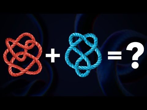
This highly visual introduction illustrates the physical and historical context of knot theory. It intuitively introduces the concept of a "knot invariant" and explains why simply looking at a highly tangled loop is not enough to determine if it can be untied into a simple circle (the unknot).

---

Why this video

Dr. Trefor provides a rigorous yet accessible transition from intuitive loops to mathematical structures. He explains ambient isotopy—the continuous deformation of space that allows us to stretch and twist a knot without cutting it or forcing strands to pass through one another.

---

Why this video

This video formalizes the topology. It defines a knot as a smooth embedding of the circle $S^1$ into $\mathbb{R}^3$. It also explains the necessity of studying "tame" knots (which can be represented by polygonal curves) to avoid pathological counterexamples like "wild knots" that possess infinite crossings.

---

Knowledge Checkpoint

• Can you explain the fundamental mathematical difference between a shoelace knot and a mathematical knot?
• What is "ambient isotopy" and why is it the standard of equivalence in knot theory?
• What defines a "tame" knot, and why do mathematicians restrict their focus to them instead of "wild" knots?

---

Module 2: Reidemeister Moves & Knot Equivalence

To work with 3D knots algebraically, we project them onto a 2D plane as "knot diagrams." This module covers Reidemeister's Theorem, which states that two knot diagrams represent the same 3D knot if and only if they can be transformed into one another using a finite sequence of three local diagrammatic moves.

Recommended Videos

Why this video

Dr. Richard Hepworth provides a clean, academic introduction to diagrammatic knot theory. He precisely demonstrates how the 3D geometry of ambient isotopy is simplified into 2D diagrammatic moves (planar isotopies plus the three Reidemeister moves).

---

Why this video

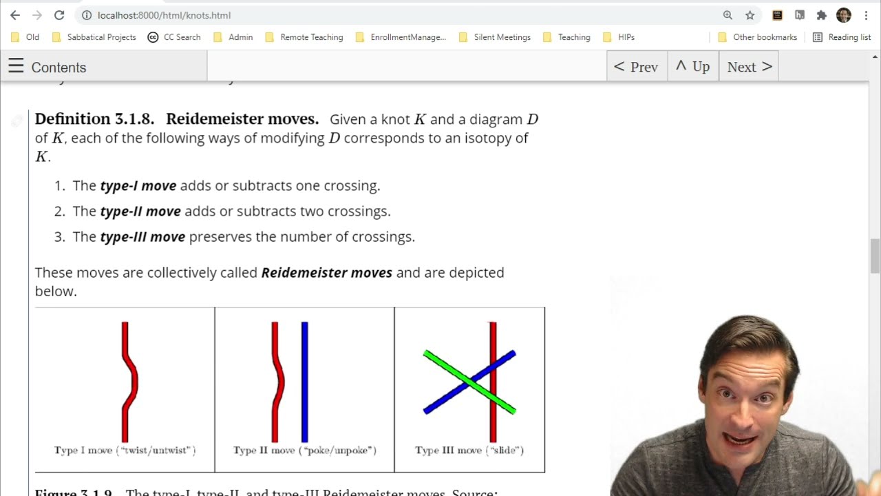
Professor Salomone offers an excellent step-by-step breakdown of how to manipulate knot diagrams. This video is ideal for beginners to visualize the three moves: Twist/Untwist (Move I), Slide-over-strand (Move II), and Slide-over-crossing (Move III).

---

Why this video

This concise video bridges Reidemeister moves to the concept of coloring. It illustrates how local changes to a diagram alter the number of strands and crossings, highlighting why we need invariants that remain unchanged under these moves to prove two diagrams are truly different.

---

Knowledge Checkpoint

• Draw and label the three Reidemeister moves: Move I (twist/untwist), Move II (poke/pull-apart), and Move III (slide across a crossing).
• If you are handed two different knot diagrams, does Reidemeister's Theorem guarantee a constructive algorithm to find the sequence of moves that transforms one to the other?
• Why is planar isotopy (deforming the diagram without changing crossing relationships) considered a "zero-th" Reidemeister move?

---

Module 3: Knot Invariants and Tricolorability

Since there is no simple algorithm to find a sequence of Reidemeister moves between two arbitrary diagrams, we use knot invariants: properties computed from a diagram that do not change when any Reidemeister move is applied. This module teaches tricolorability and its powerful algebraic generalization: $p$-colorability and the knot determinant.

Recommended Videos

Why this video

This video delivers a complete proof showing that tricolorability is preserved under all three Reidemeister moves. Understanding this proof is critical because it models how mathematicians verify that any proposed property is indeed a topological invariant.

---

Why this video

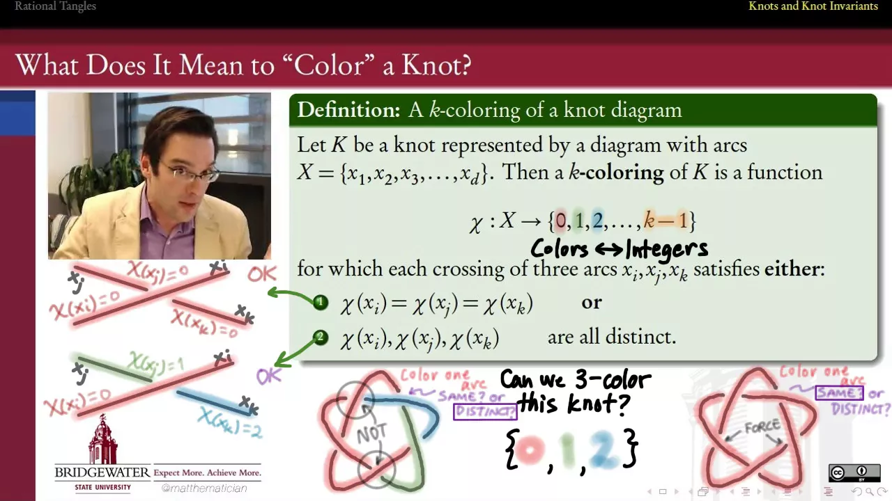
Addressing the $p$-colorability gap: This video generalizes tricolorability (which is arithmetic modulo 3) to $k$-colorability (coloring mod $k$). It provides the formal definition of labeling arcs with integers from $0$ to $k-1$ and proves that this algebraic system is a robust knot invariant.

---

Why this video

Addressing the algebraic formulation gap: Legendary topologist Louis Kauffman demonstrates how to turn a knot diagram into a system of linear equations. At each crossing, the over-crossing arc ($a$) and the two under-crossing arcs ($b$ and $c$) satisfy the algebraic relation: $2a - b - c \equiv 0 \pmod p$ Kauffman shows how this translates coloring into a rigorous algebraic framework.

---

Why this video

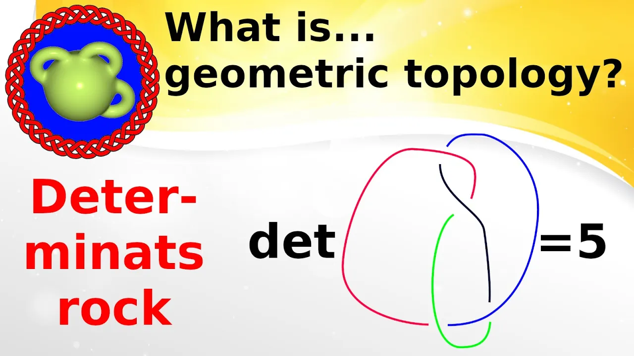
This video explains how to use linear algebra to solve the coloring problem. Instead of guessing colors, you construct a matrix of crossing equations, take a minor, and calculate its determinant. The knot determinant reveals exactly which primes $p$ allow the knot to be $p$-colored.

---

Knowledge Checkpoint

• What is the formal definition of a tricolorable knot? (State the rules for colors meeting at a crossing).
• Translate a crossing where arc $x_1$ crosses over arcs $x_2$ and $x_3$ into its mod $p$ algebraic equation: $2x_1 - x_2 - x_3 \equiv 0 \pmod p$.
• How does computing the determinant of a knot's crossing matrix determine which $p$-colorings are possible? Why is one equation always redundant?

---

Module 4: The Kauffman Bracket

To distinguish more complex knots, we need stronger invariants. Louis Kauffman developed a state sum model that maps knot diagrams to Laurent polynomials. In this module, you will master calculating the Kauffman bracket by hand and learn how it interacts with the Reidemeister moves.

Recommended Videos

Why this video

Dr. Hepworth introduces the three axioms of the Kauffman bracket $\langle D \rangle$:

1. $\langle \text{unknot} \rangle = 1$
2. $\langle D \sqcup \text{unknot} \rangle = (-A^2 - A^{-2})\langle D \rangle$
3. The skein relation that splits a crossing into $A$-type and $B$-type smoothings.

---

Why this video

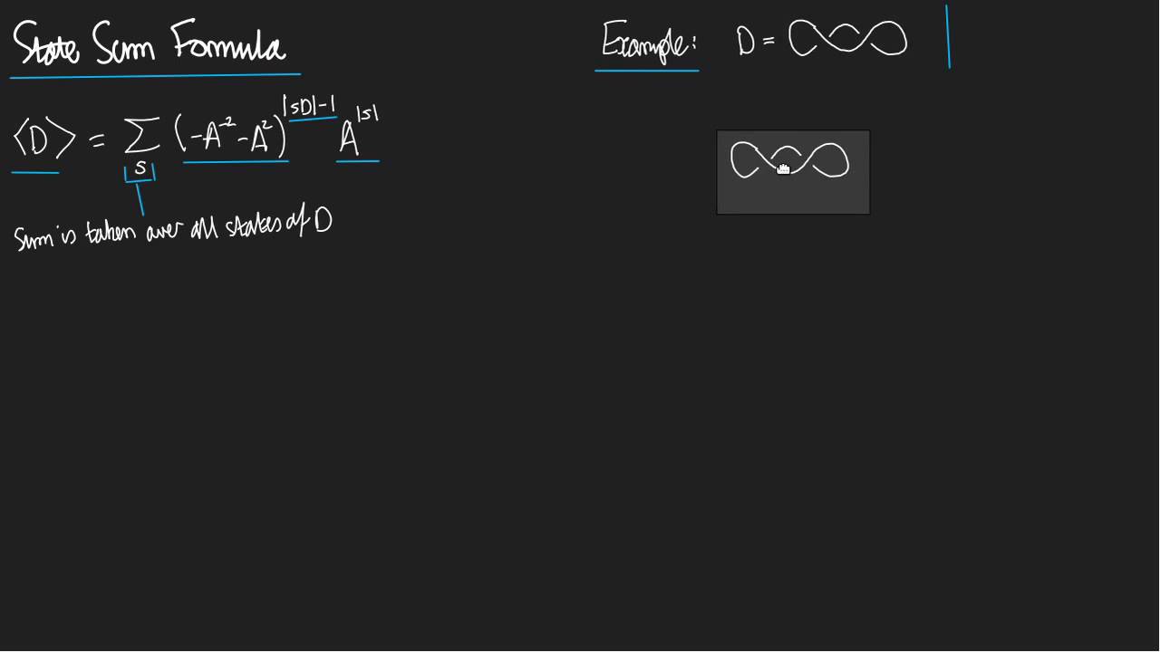
Addressing the step-by-step hand calculation gap: This video teaches you how to compute the Kauffman bracket of a knot diagram using the state sum formula. For a diagram with $n$ crossings, Hepworth demonstrates how to expand the diagram into $2^n$ distinct states (configurations of non-intersecting loops), assign weights, and sum them to obtain the final polynomial.

---

Why this video

Bridging to Module 5 via Writhe: This crucial video proves that the Kauffman bracket is invariant under Reidemeister Moves II and III, but fails under Move I (introducing a factor of $-A^3$ or $-A^{-3}$). Hepworth introduces writhe (the sum of signed crossings of an oriented knot) to measure this twist and shows how it will be used to fix the bracket's Move I sensitivity.

---

Knowledge Checkpoint

• Resolve a crossing using the Kauffman bracket skein relation: $\langle \lambda \rangle = A \langle \asymp \rangle + A^{-1} \langle \big( \rangle$
• For a knot diagram with $3$ crossings (like the trefoil), list all $2^3 = 8$ states, count their loops, and write down the full state-sum calculation.
• Why is the Kauffman bracket considered a "regular isotopy" invariant rather than an "ambient isotopy" invariant? (Hint: Think about Reidemeister Move I).

---

Module 5: The Jones Polynomial

By combining the Kauffman bracket with the geometric concept of writhe, we can eliminate the sensitivity to Reidemeister Move I. This produces the celebrated Jones Polynomial, an ambient isotopy invariant capable of distinguishing chiral knots (like the left-handed and right-handed trefoil) where previous invariants failed.

Recommended Videos

Why this video

Dr. Hepworth formally defines the Jones Polynomial. He introduces oriented knots, where each strand has an assigned direction, allowing us to assign a sign ($+1$ or $-1$) to each crossing.

---

Why this video

This lecture provides the mathematical normalization formula: $V_L(t) = \left( (-A^3)^{-w(D)} \langle D \rangle \right)\Big|_{A = t^{-1/4}}$ Hepworth demonstrates how multiplying the Kauffman bracket by $(-A^3)^{-w(D)}$ (where $w(D)$ is the writhe) perfectly cancels out the scaling factor introduced by Reidemeister Move I, resulting in a true topological invariant.

---

Why this video

This video focuses on calculating the Jones polynomial using oriented skein relations: $t^{-1} V(L_+) - t V(L_-) + \left(t^{-1/2} - t^{1/2}\right) V(L_0) = 0$ This recursive method allows you to find the Jones polynomial of complex links by breaking them down into simpler, known links.

---

Knowledge Checkpoint

• Determine the sign of a crossing: when is a crossing designated positive ($+1$) vs. negative ($-1$)?
• Compute the writhe $w(D)$ of a standard three-crossing trefoil knot diagram.
• Why does the Jones polynomial succeed in distinguishing the left-handed trefoil from the right-handed trefoil, whereas tricolorability fails?

---

Course Map

---

Key People Index

• Kurt Reidemeister (1893–1971): German mathematician who proved that knot equivalence in 3D is homeomorphically represented by three local moves on 2D diagrams.
• Louis Kauffman (b. 1945): American topologist who introduced the Kauffman bracket state-sum model, simplifying the computation of the Jones polynomial and bridging knot theory with statistical mechanics.
• Vaughan Jones (1952–2020): New Zealand mathematician and Fields Medalist (1990) who discovered the Jones Polynomial, establishing a profound connection between von Neumann algebras, mathematical physics, and knot topology.
• Peter Guthrie Tait (1831–1901): Scottish physicist and pioneer of knot tabulation, whose conjectures regarding crossing numbers and alternating knots stood unproven for over a century until resolved by the Jones polynomial.

---

Final Self-Assessment

Complete this checklist to verify your mastery of the curriculum:

• Definition: I can mathematically define a knot as an embedding $K: S^1 \to \mathbb{R}^3$, explaining why $S^1$ represents a closed loop.
• Projection: I can draw a valid knot diagram, including proper gaps at crossings to denote over- and under-strands.
• Reidemeister Moves: I can transform a trivial loop diagram containing redundant twists into a clean unknot circle using only the three Reidemeister moves.
• Tricolorability Proof: I can explain why a knot is either tricolorable or not, and prove that if one diagram of a knot is tricolorable, any diagram obtained by a Reidemeister Move II remains tricolorable.
• Generalization: I can define $p$-colorability for an arbitrary prime $p$ using modular equations.
• Matrix Representation: I can construct the crossing matrix of a knot diagram, calculate its determinant, and identify which primes $p$ allow non-trivial colorings.
• State Splitting: I can correctly perform $A$-smoothings and $B$-smoothings at any crossing of a knot projection.
• Kauffman Formula: I can write down the state sum formula for the Kauffman bracket, explaining how the term $(-A^2 - A^{-2})$ arises when removing disconnected components.
• Writhe Calculation: I can assign orientations to a knot diagram, determine the sign of every crossing, and sum them to compute the total writhe $w(D)$.
• Jones Polynomial Computation: I can combine the Kauffman bracket and writhe of a knot diagram to calculate its normalized Jones Polynomial $V(t)$.
• Chirality Verification: I can explain how $V(t)$ for a mirror image is obtained by replacing $t$ with $t^{-1}$, and use this to prove that the trefoil knot is chiral (not equivalent to its mirror image).