1D Dynamical Systems: Linearization & Bifurcations

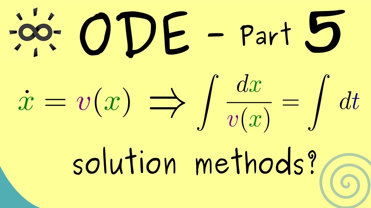
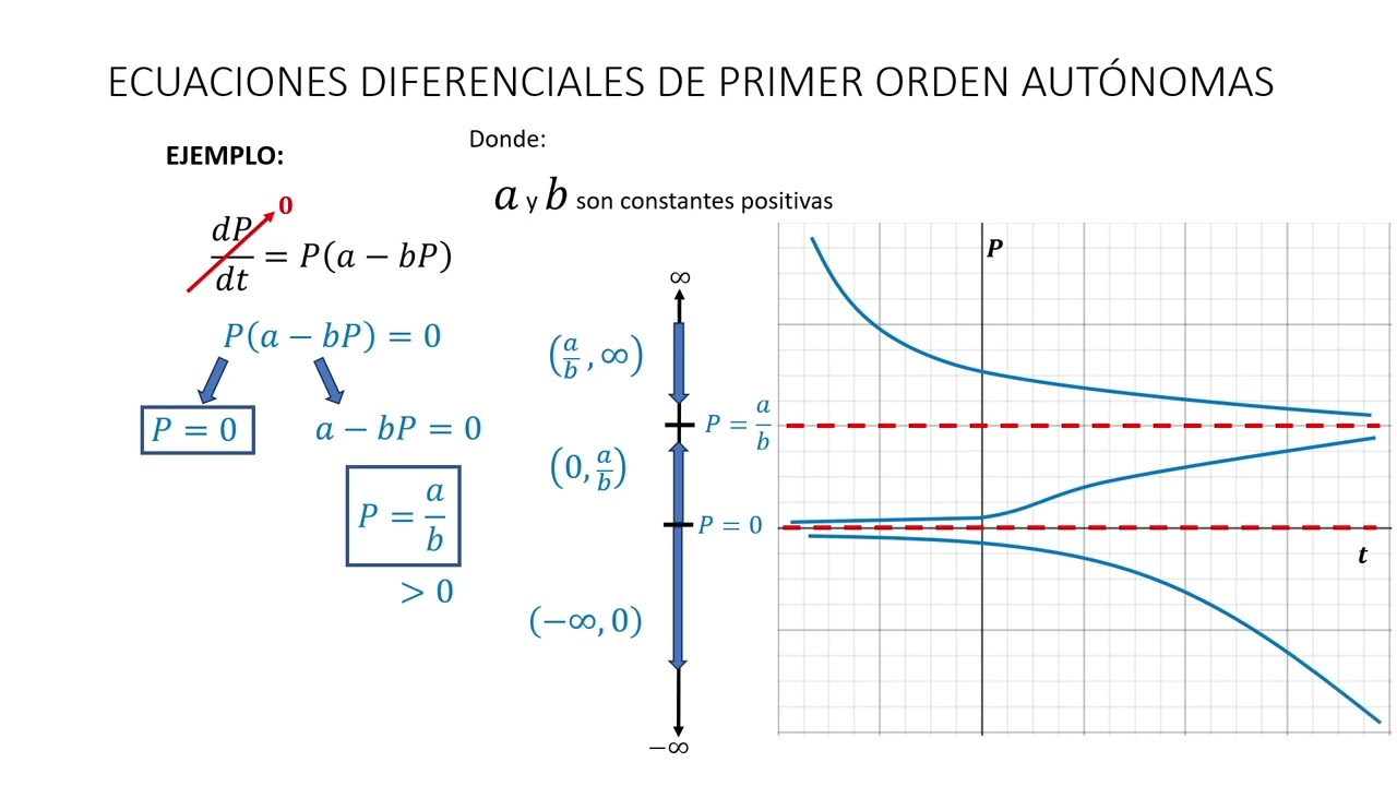
[00:00:00]begin we um talked in the first lecture about uh the history of dynamical systems and The Logical structure of the subject and I tried to give you an overview of what the whole course will be about and we then got into a little bit of math about one-dimensional systems which are uh dynamical systems of the form x. X is just a real number so last time we looked at this class of systems where X as I say is just a real number and we said that you could try to solve them analytically but often it will be impossible to do the integrals that will arise if f is a nonlinear function you may not be able to do the integral that would come up if you use separation of variables on the other hand pictures are are really easy to use in this context and that's going to be the approach we'll take all semester so um the approach was to just draw the graph of this function f you know so maybe it's some nasty looking function like that but we said understanding the dynamical system is pretty easy because all you do is think about a imaginary particle that's moving on the X AIS as a function of time and then this equation would say its velocity is given by this function f ofx so that would mean that when the particle is here its velocity would be given by this x dot which is positive so it'd be moving this way and actually this particle will always be moving to the right except when it's over here where x dot is negative then it would move to the left and then we pointed out that there are these special places where the function crosses the axis like here which we called a fixed point because if you happen to be there then you won't move and that would be in physical terms an equilibrium State for the system so we can see what the long-term behavior of this system is everything that starts to the right of this point will go out to infinity and everything on the left will go out to negative infinity and we could do that without doing any analysis just looking at the picture so that was the approach from the first uh discussion and I want to go a little more deeply into that now uh yes is it ever possible to reach a fixed Point uh the question was is it ever possible to reach a fixed Point um well it depends on the nature of the function f so for the functions that we're going to consider in this course which have um the property that they're continuous and continuously differentiable then um it will not be possible to reach a fix point you could approach it and and get closer and closer and so to speak get there at infinite time but if you want to get there in finite time um you can't do it with the functions we're going to consider it is possible there are you can make constructions of functions that have infinite slope for example and then you can actually reach a fixed point in finite time but for the most part we won't deal with those kind of functions was there another question so then uh having mentioned this graphical method and then saying that we're not going to do much about analytical methods I do want to touch on one analytical method that that's quite easy and will be helpful to us so this is discussed in section 24 of the book and it has to do with the idea of linearizing around a fixed point so here's how it goes we're going to examine the Dynamics close to a fix point which I mentioned last time we'll tend to use the notation xstar for a fix point and you know like in this little example this is the fix point that is fixed points satisfy F of xar is zero the velocity is zero there and so if we look in the neighborhood of the fix point that is not right at the fix point but on either side of it we want to see whether a little deviation will grow as it does in this case in which case we would say that the fix point is unstable or does it decay bringing us back closer to the fix point in which case we would say it's a stable fix point and so to do this we'll say let's let um our X of T be xstar but then plus a little deviation what that I'll call by the Greek letter Ada where we're going to assume that ADA is very small in magnitude and um I'll make it clearer in a minute what I mean by very small but for now just think of some very tiny perturbation and and then um we want to derive an equation now for Ada to see does this deviation grow or Decay so to do that use a differential equation um x dot with this Choice becomes xar plus Ada all Dot and since xar is a constant it's derivative is zero but Ada is not constant so we get a to dot on the other hand it's supposed to be f ofx and that means it's F of xar plus Ada now at this point everything is exact but still not so clear what's going on because this F is this complicated nonlinear function so here's where we invoke the idea of linearizing by saying that um let's use uh Taylor's formula here that is I'm just going to assume that this function f is smooth enough that I can write down the tailor series approximation to it in the neighborhood of xar and so um this would give us then f of x Star Plus a fime at xar plus the next term would be a^ 2 over 2 uh you know two factorial which is two FP Prime at X star and then there are higher order terms of order Ada cubed and so on but let's just leave it at that for now there's another question yes um the question was are we always going to assume that our functions F have convergent tailor series which would be in the jargon of pure math to say that we're only going to work with analytic functions for the most part that's true we will mostly work with analytic functions we'll also take the attitude that this is an applied Math course not a pure Math course and we're not going to worry about smoothness that is um functions are as smooth as we need them to be to do whatever manipulations we do on them and the the feeling is if we're going to get in trouble we'll recognize that in the course of our work so I'm not going to be um doing rigorous math with careful smoothness assumptions I I do try to refer to the smoothness assumptions I need in the book if you want to look into that kind of thing more deeply but yes so I'll just be very Cavalier in the style of a physicist or engineer where I just assume everything has a tailor series when I need to um is there another question okay so all right so let's look at this expression over here on the right um well first of all F ofx star notice is zero because we said we're not just linearizing any old point we're linearizing around a fixed point so we already have F ofx star is zero as I mentioned over here okay so that gets rid of that constant term this term is linear in Ada so this is why we speak of the linearization it's proportional to Ada and although this looks like some complicated thing frime of X star keep in mind that it's really just a number I mean it looks like a function but it's a function evaluated at a specific point x star and all it's really telling us is the slope of F at the fix point which in this picture would just be you know whatever that slope is fime at xar so I have some number times Ada and then some other number times Ada squared and you've probably seen arguments like this elsewhere that we said Ada is very small and so at this point we want to neglect the Ada squar term because if Ada is small a is really really small we want to neglect Ada squ compared to Ada and so that's the idea of linearization that um we want to neglect this quadratic term you know this term now you have to think about that for a second um also I'm going to neglect for the same reason but even more so all these higher order terms in Ada but um still you have to think about it just for one second are we sure we can neglect this term compared to that term the the answer is yes we can as long as this F Prime is not zero if it's zero then this term is not even there and then this would be the leading term in the expansion in that case we better not neglect it so uh but otherwise we can so if fime at X star is not zero the term um this term in magnitude is much greater than this term you know for small a and so um for that reason we'll just neglect that ADA squar term and that gives us the linearization so I'll frequently use this notation this is Big O that's not a zero that's the capital O that stands for the order of and neglecting the terms that are of the order of a to squar yields the linearization of the system at the point xstar which is the system essentially that ADA dot is a constant time Ada where this constant R is this number f Prime at X star the slope at that point that we've been talking about and so you see this is a very easy little linear differential equation that we know much about from previous either calculus or differential equations courses that is that just produces exponential growth or Decay depending on if R is positive or negative so you would get exponential growth a to grows like whatever the initial Ada is times e to the RT actually I might as well say equals because it's not just approximately it really is equal for the linearization um so we get growth if we have R greater than zero and then we have Decay if R is less than zero and notice that that's consistent with our picture above that is we have here in this context um we see a positive slope and notice that that point is unstable graphically but it's also unstable analytically because deviations are growing exponentially fast at least for small Ada so that's um the idea of linearization very easy in one dimension we'll also be doing it later in the course in two dimensions and three here it's quite quite I don't know hardly even been worth bothering but okay uh though you may be wondering what about if frime of xar is equal to zero this caveat I have here what if it is zero what would we do then so in this case there's uh no information from linearization [Applause] by that I mean that if I find F Prime is zero at a fixed point that tells me nothing about the stability of the point it could be stable or unstable or even a kind of hybrid situation where it's half stable so just to give you a few examples of what I mean by that um consider these four different systems x dot is x s um x dot isx2 x dot is X cubed or x dot is negative X cubed all of those have fix points at zero right xar equals z is a fixed point for all of them as you can see by just plugging in zero on the right hand side you get X do is zero so it's a fix point and also notice that um we have F Prime at X star which is fime at zero would be zero in each case and yet if we just draw the pictures we can see easily that they have four different stability types in other words just knowing a zero uh just knowing that the derivative is zero at at the fix point we anything sort of as possible as far as stability let's just see what goes on in detail here let's take the top One X doal x^2 so again rather than solving it analytically where we would just draw a picture um X doal x^2 we have x dot here here's X you draw the parabola X squar and then you see that over here x dot is positive so you go this way but also over here x dot is positive so you're still going that way and that means that this fix point is kind of strange we haven't talked about it yet but this a good time to do it we would approach it ASM totically from the left and so our convention would be to fill that in because it's stable to approaching from the left on the other hand it's unstable from the right if you make a perturbation away from the point that perturbation will grow so this is a half stable fix point it's stable from one side but not the other and likewise if you look at X do = x^2 that would have this kind of picture where now it's you know the opposite it's now um stable from the right but the left and if you do x dot is X cubed um well X cubed has a graph like this and well let's see so this is now positive over here negative over here so we just have an honest to God unstable fix point in that case and finally if x dot is negative x cubed well then the graph looks like so and it's a stable fix point now it's not stable in the same analytical sense as our original um stable fix points which were exponentially stable that is you had exponential decay toward them here the Decay would be much slower than exponential it'll actually turn out to Decay to zero like a power of 1 overt you'll have to you could check the details if you're curious about that but so you have algebraic relaxation which is very slow and Pokey compared to exponential but anyway it is still stable from the graphical sense so is there any question about what's been shown or what the point was of of this so far and I guess I would say the bottom line is if you want to figure out stability information at a point where fpre is zero just draw the graph um and that'll tell you what's going on or you could if you really insist you could do the tailor series out to a higher order to x^2 or X cubed or I guess in my notation Ada squ or a cubed but I really do think that's the wrong way to think I I think you should look at it as pictures um okay let me do one little example of this and then move on we talked about the logistic equation for population growth which you'll remember is x dot is rx 1 - x over K where X is um the population of organisms R is their growth rate and K is the carrying capacity how many um organisms the the little system can support the sort of I hesitate to call it an ecosystem it's just this one population but anyway um so looking at this with linearization we can see that X do equals z when either xar is zero or xar is K those are our two fix points and then if we wanted to figure out their stability we could look at F Prime at X which um I have to take DDX of this so I'll get R and then minus this is rx^ 2 over K differentiating that gives me 2 RX over K and then if we calculate F Prime at one of the fix points at zero it's just R which is positive we're assuming R is positive it's a positive growth rate and so this tells us that xar equals 0 is unstable whereas the other fix point if we look at k then we get r - 2 r k over K and the K's cancel out and this is R so this is less than zero and so X star equal K is stable right remember the Criterion negative fpre gives us stability positive gives us um oh I guess my notation is a little nasty there isn't it because I'm calling that R but that's a different R from this R uh but okay ignore that we're looking at fime at xar so anyway these are conclusions are consistent with what we said graphically where the logistic equation has um this kind of picture of X do versus X where we saw that this point at K really is stable and the origin really is unstable okay so linearization gives us the same information any question about that I I think then I'm going to leave linearization and talk about a few more things in this um second chapter and then get into the third chapter which is where things start to get interesting [Music] okay so um the question came up earlier about can you reach a fix point in finite time or can you ever reach it at all and um so this ties in with this a pure math notion of the existence and uniqueness theorem for ordinary differential equations so let me just comment on it I I said something briefly a few minutes ago you could read about it in section 25 and I don't really want to dwell on it just to say one thing which is that there's a theorem that you would prove in a rigorous differential equations course that says that the solutions to X x doal f ofx um do exist and they are unique if I mean these are not the best possible conditions I'm going to give there are milder conditions that would also ensure these existence and uniqueness but for us it's good enough to say um if we have F continuous and if we have fime of X continuous so that's when we would say that f is continuously differentiable if it has these two properties and so under these assumptions you can prove then that the solutions to the differential equation exist um now that doesn't mean they exist for all time they might exist only for a very short time after you start them from some initial condition so there's no guarantee about existence for all time but um it does the solutions do exist in some possibly small time interval around time equals z and um there's only one solution so that's sort of what we want I mean that's what we've been assuming in the way we draw the pictures but if you relax these conditions too much then you can get some pretty weird pathologies um which I've mentioned some examples in the book but they're not going to really concern us so okay so that's one uh thing and then the other that I want to mention this a little more interesting I would say is this remark which is touched on in section 26 of the book which is that if you ask what can these one-dimensional systems do what kind of behavior can they have they're very limited in what they can do that is um if we ask what's the possible behavior of X of t as T goes to Infinity for these 1D systems X do equals F ofx then the only things that can happen are either as we saw in the earliest example that the um where had that one unstable point and trajectories either went out to plus or minus Infinity you can have that so either X of T goes out to Infinity in one or the other direction or um X of T approaches a fixed Point that's it and and in particular what's not possible is anything like an oscillation a periodic solution even a damped oscillation is not possible so it's impossible to have something whose time series would look like this or even um a more period you know like a true periodic one those are not you can't see that in in this class of systems um and you certainly can't have chaos so these have really kind of boring long-term Behavior they just approach an equilibrium point or go out to Infinity you might say how do I know that what about if I think up a really clever F you know are we sure that it's not possible to to do something like this yes we're sure it's it's true for very easy topological reasons so let's see why the reason is that um all the trajectories or Solutions whatever you want to call them increase or decrease monotonically or stay fixed and I don't really know quite how to give you a proof of this in the spirit of the course where I'm not really proving things but the the intuition is just draw whatever smooth F you can think of you know I mean as we said under a a a positive hump like this you just move monotonically to the right till you hit a fix Point here here you would move monotonically to the left what's the problem I mean why can't you oscillate maybe think of it that way what would it mean if you if you did have an oscillation it would mean that pick some value of x that you're interested in remember this is the x axis this is x dot suppose I thought there was an oscillation where I go through this x value once you know going that way and then when I oscillate I come back and go this way to the left that would mean that the vector field is not well defined here because it would at sometimes be pointing to the right when I'm going that way it would also be pointing to the left when I'm coming back and that violates the single valness of f right I mean if f is a function it only points one way at each point so you can't go two ways through the same point that's all there is to it um so there are no oscillations in one dimension now you might ask wait a second this sounds ridiculous of course I've heard of the simple harmonic oscillator it moves on the x- axis it oscillates so what's the point yeah that's the point is that the simple harmonic oscillator is not a first order system it has X double dot right so the X double dot means that to write it down geometrically we're going to need two Dimensions one for x and one for x dot and that'll be studied later in the course those are second order systems so so if you want to think purely mechanically or physically these first order systems you should think of as just a force being balanced by damping by a dash pot there's no inertia there's no X double dot term so if you you know have some kind of weird nonlinear Spring Pulling on a a mass that is is so tiny it has no inertia and it's just moving through goop of tremendous viscosity so it's very overdamped that thing is not going to oscillate that's just some complicated shock absorber that's just going to just go back to its equilibrium so I don't know if that's clear or not do you want to ask anything before we move off of that topic okay so there's yeah there's no chance of overshoot for these systems no oscillations all right so let's leave chapter two and move on to chapter 3 actually let's stay here okay now chapter 3 uh is pretty substantial that brings up the very interesting and important topic of bifurcations in the simplest possible setting still talking about these one-dimensional systems later in the course we'll talk about bifurcations in two-dimensional and higher dimensional systems but for now let's just focus on these flows on a line so all right what is a bifurcation well um think about some system that has a parameter in it some kind of Knob you can turn then uh like for instance I imagine this picture here's a here's a little support and then I put some kind of heavy block on it and I ask can that um block just stay in this vertical position maybe if the support is strong enough but now suppose I make a really big block I'm putting some gigantic Boulder on there it it seems unlikely that this thing is going to be able to hold the heavy weight and it's going to you know tend to well this this straight structure will Buckle right it'll Bend to either side it'll either Buckle like this and the whole thing will come crashing down or it might Buckle like that but so the straight solution will not be stable anymore and we'll have something else going on so this is typical of a bifurcation that you've Chang change some parameter in this case the stress or the load and you get a dramatic and Sudden Change in the response of the system as you change this parameter so as a parameter changes um for us speaking about Vector fields on the line as models of differential equations the um as a parameter changes the qualitative structure of the vector field may change dramatically for example um a fixed Point might be created or destroyed or they might change their stability so by qualitative change I don't just mean like you move a fix Point around I mean means something much more dramatic than that that it actually just vanishes and now it doesn't exist anymore or it um changes from stable to unstable or something like that and so a a change of that type is what we would call a bifurcation and then we also have the further language of a bifurcation point or value that's the value of the parameter at which the change occurs so as I tried to hint with that example with the block on the little um straight you know drinking straw or whatever that thing was um these are relevant to science so you probably depending on what field you study you've run into bifurcations a lot maybe not by name um in fluid dynamics if you have a a flow that's laminer and you start turning up the Reynolds number that flow might start to become wavy in a bifurcation or then if you keep going high enough it may become turbulent those are those are important and still somewhat mysterious bifurcations if you're studying say heart rhythms like people in our vet school work on there's the normal heart rhythm which hopefully you're experiencing as we speak and then if you have a bifurcation to arhythmia that that would be bad especially if it's the deadliest kind of arhythmia called ventricular fibrillation in which case we only have a few seconds to save you so um the study of bifurcations is pretty important in all parts of science and so I want to begin our discussion of them with just a few little easy mathematical examples without any scientific content um just to get warmed up and then in later lectures we'll talk about some some pretty interesting scientific examples one from mechanics and one from um population biology and we'll have many more throughout the course so roughly speaking then these are models of instability ilities or sudden transitions so models of instabilities um Transitions and so on okay but first let's just get warmed up as I say with um a few of the basics so the most basic one is a a bifurcation that creates fix points out of nothingness uh it does it in pairs it's almost like in physics when they talk about a particle and an anti-particle coming out of the vacuum this is something like what we have except for us it'll be a stable and an unstable Point coming out of the vacuum so it's for reasons that are not clear at this stage in the course but will be clear I hope later in the course this is called the saddle node bifurcation um the language doesn't make sense yet because saddle points only exist in two and higher Dimensions so we don't have room for them but this is the analog of what we're going to see in higher dimensions and we still call it saddle Noe so it's the basic mechanism for the creation or destruction of fixed points and so here's a standard example that is this is probably about the easiest system that has the phenomenon in it let's look at x dot equals R plus X squar where this R is um what I'm thinking of as my control parameter that is if I'm an experimentor R is the knob that I can turn by changing something in my apparatus or whatever so I have control on R and now I want to watch how my system behaves and so when R is negative then if I look at my x dot versus X picture notice um of course this is a the graph of the right hand side is a parabola but it has an intercept of r on the vertical axis so when R is negative it would look like that and it's a Parabola opening upward and now you can see that you know from our techniques that we've got negative x dot here positive here and um positive over there telling us that this is a stable fix point and this one is unstable so right now we have two fix points of opposite type now imagine that we start turning the knob and R is being brought closer to zero so imagine that R is only slightly less than zero then you'd have a picture like this with the parabola just barely going underneath so it's still negative but but close to zero and notice what has happened our our fix points have gotten much closer together so if you were watching a movie of this you would think of lifting up the parabola gradually and these two fix points these intersections would be moving towards each other ominously right and then at R equals z baboom they're going to hit and so they would Collide and then you would have this picture that we discussed earlier where it's now just X dotal x^2 with that funny half stable fix point you can now kind of understand by the way where that funny half stable fix Point came from we were catching a system at the moment of bifurcation and the the stable and unstable ones have merged and that's why you've got this half and half character here and then finally when R is greater than zero well now the parabola is above the axis and the flow is everywhere to the right it's just there there are no fixed points they're gone so it's as if after the Collision of the stable and unstable point they have now annihilated each other and they're gone um and so we went from two fix points to one of this weird hybrid type and then zero all by continuously changing R okay so I hope you would agree that's a qualitative change here's a system with no fix points and here's one where you can get stuck in two places yes do stable fix points arise oh half stable I'm sorry do half stable points arise only as a result of bifurcations I think that would be fair to say yeah they don't you wouldn't normally I mean if you have implicitly there would be some parameter in the problem which if you changed it it would take that that half stable fix point and make it either into nothing or into something like that or it depends on how the parameters introduced we'll see other mechanisms for creating half stable points besides this one but I think it's safe to say say yes it would it's um always a result of some bifurcation is there another question okay so that was the saddle node bifurcation and there's a standard way of representing it that is you could show these the sequence of pictures but there's a little um diagram that everyone draws called the bifurcation diagram that encodes all of this in one picture so a bifurcation diagram would be something like um draw plot the curves of xstar versus the control parameter R where we think of r as the independent variable we're that's the thing under our control and then we watch what xar is doing so in this case by just setting X do equal to Z to find the fixed points we see R plus the fix point xar squar is zero and so the graph of that let me just call this x not quite X star because the xar is going to appear as the curve um xar would be plus or minus what the Square < TK of R and so over here it would look like this now I'm going to just draw a dotted line for now because I want to concentrate one of those is is going to represent a stable fix point and one represents an unstable fix point but let's concentrate for a second to see which one is which how do I tell which one of these is stable is this Branch stable fixed points or is this do you see how to think about it you want to put up your hand yes you have looks like you have an idea negative yes the comment is the stable fix point is the negative one so in fact in this picture this must be the stable Branch right it's always the negative one that was stable so our notation is that we use a solid line sort of In The Same Spirit as a solid dot for the stable branch and then we would use a dashed line for the unstable one so to make it a little more visible let's just make some big dashes here and it's also sometimes helpful although not really necessary to um draw some arrows that is we know that we're well at a think of a holding R constant then that would mean that um you just at some on some vertical line in this picture that represents the x- axis at that choice of R and so you would say like in this slice you'd be going this way and this way and like that so you can add that if you want now it's a little distracting the x- axis is a mean sorry the r AIS is a meaningless artifact in this picture which probably shouldn't really even be there um but okay so there it is and then what else uh well and then over here we're just going this way up up up okay so anyway that's the bifurcation diagram for the saddle node and people use other words for it sometimes it's called a turning point bifurcation because in this picture it looks like this branch is turning around and then becoming unstable or it's also sometimes called the fold bifurcation because it looks like you took a straight line and folded it to make this Parabola so you'll hear words fold or turning point but I'm going to call it the saddle node any question about this yes the dashed line here refers to these unstable points so this unstable point you know if we calculate it this is at X star is the positive square TK of R and so that's why it's up here at the positive square root of negative R this doesn't mean flow on the picture I'm just indicating it maybe I should make it look like this who there any other um comment or question okay so that's that's as I say the standard example like the most pristine example of a saddle node bifurcation now in real life um or in typical practice you would not see it so cleanly so let me show you a type of question where um it's more like what you might encounter in a in a in your own work let's look at this example suppose I give you this differential equation x dot is r + x minus natural log of 1 + x okay so there's something fairly nasty right hand side nonlinear term log of 1 + x um we want to analyze that as a function of r what's going on with that system as a function of r so you could you know your first thought is well let me figure out what the fix points are since they dominate the behavior of these one-dimensional systems and so the fixed points would [Applause] satisfy well the right hand side has to be zero so we have r + x equal log of 1 + x or those I guess we would put as X Stars and already you know you kind of feel like well it's not so easy to solve for x as a function of r in fact I I tried to make it so that it's impossible that is you can't invert that I don't think algebraically for X of R so um if you're stuck in this old analytical way of thinking you feel paralyzed at this point and you just give up but of course we're graphical not Analytical in this course and so we would say that's actually pretty easy to understand because um I can draw the graph of both of those and then figure out what's happening that is let me even though I can't solve for xar of R um but a simpler approach is to just use a graphical method where what we're going to do is plot both of these functions let's plot y = r + x and plot y = log of 1 + x and so you'll remember on the first day I said that you have to be good at Curve sketching in this course it's because of things like this you if you had to use your graphical calculator to draw y = log of 1 + x you'll just be slow and you'll be at a disadvantage so try to have the basic functions and their shapes in your head or at least be good at figuring out what they look like all right anyway maybe maybe you do know how to draw them both and so log of 1 + x is I'm going to just look like the log function except shift it over so it's sort of like this and I'm thinking of this as y now this is not x dot okay that vertical axis just represents some madeup axis y that I'm using to graph these two functions and the reason for doing that is well log of 1+ x is there r+ X is a function with a its graph has got a slope of one and an intercept of r right just a straight line with a slope of one like that and you see that these two um curves don't intersect at the moment so what does that tell us well if they don't intersect it means that this is not equal to that for any X so we don't have any fixed points when R is like the r in the picture on the other hand you could imagine as you start changing R which would mean sliding the line down but keeping its slope at one you can see that this line is going to bang into the curve at some point and we could draw a sequence of different pictures here it's almost hitting here it's tangent here it has hit and now has two intersections so do you see that that's really the same scenario as what we talked about that there's there's no roots then there's one root and then there's two went from zero to one to two fix points that's what happens in the saddle node bifurcation so in fact you can now see that this system does have a saddle node [Applause] bifurcation saddle node bifurcation occurs when um what would be the condition in geometric language anguage when what happens is it is it obvious you want to say go ahead you could say in the back yeah well if there if the line intersects the curve tangentially right so if there's a tangential intersection now we have to think about um when does that happen and so it's when two things happen on the one hand we have that condition which says that an intersection occurs and it should be a tangent intersection meaning that the line and the curve have the same slope at the points where they meet at the single point where they meet so it's not just that this is true but also DD X of r + x should equal DDX of log of 1 + x you need both the tangency condition is the second one right they intersect with the same slope and so now we can calculate where does that occur in the sense of where in the parameter R and where in X so we already know that we can't really solve this first equation the second one is going to be easy so let's take those derivatives and we get 1 equals derivative of log of 1 + x is 1 over 1 + x and so that has a solution xal 0 at the bifurcation and then the corresponding value of R is given by r + x = log of 1 + x you know when X is zero so this says R is equal to log of 1 which is itself zero so um let me call it r subc for r critical like happening you know that's the critical value of R um critical or bifurcation value and notice I I my picture was actually pretty good that is it looks like it's occurring at Ral 0 xal 0 that we have a tangent intersection and I tried to draw it reasonably correctly one last thing about that um now that we know that the bifurcation occurs at 0 0 in this picture let me show you what happens if we expand the vector field around 0 0 so that is notice that um so near the by ication so near the bifurcation at XR equals 0 0 x dot let me do a little tailor expansion on the x dot itself and keep only the the leading terms in R and X so actually maybe it's clearer to write it this way let's just reproduce What x dot is it's r+ X - log of 1 + x but then keeping the leading behavior in both R and X the r we don't want to get rid of even though it's small we got to keep something that tells us about R but then hopefully you remember that log of 1 + x um has a McLaren expansion which is what it's x - x^2 / 2 + x Cub over 3 like that I think is that right yes that's right um valid for X less than one in absolute value okay and so if we just think about very small X then this is behaving like r + x minus and then using this expansion x - x^2 / 2+ X Cub over 3 Etc which simplifies to notice the X's cancel out and I get R um + x^2 /2 and then there are other terms which are of Order X cubed and higher but those are negligible compared to the X squ term what I'm trying to show you here is that near the bifurcation we get a um Vector field that looks familiar right r + x^2 forget about the two this looks like when we did the standard example for the saddle node we had r + x^2 we're getting that same thing again near the bifurcation and so um people refer to this r+ x^2 example as a normal form and there's a whole theory about you know what the vector field will look like near a saddle node bifurcation that gets Technical and I don't want to really give you a precise statement of it but in the crudest sense the statement is something like that near a Addle node the Dynamics always looks kind of like a constant time R plus a constant time x^2 you know plus or minus a constant time x^2 that's the the generic Behavior near a saddle node and that's one reason why we're studying these simplified standard examples because they're very typical want to ask anything about that before we I want to show you one or two other bifurcations before we quit um okay yes di like sidea the bifurcation diagram will pretty much always look like a sideways Parabola it won't be exactly a parabola only right near the bifurcation like if you drew the bifurcation diagram for this it would involve it would reflect that logarithm so it wouldn't give you a perfect Parabola but yes so we'll have a bend and it will look qualitatively like that it might be bending this way or it might be bending that way you have to check the details is there another question okay so let's talk about two other bifurcations that come up frequently there is quite a bit of uh jargon here in this part of the subject that is these bifurcation have not so memorable names and we're stuck with that um different Sciences were developing bifurcation Theory at the same time people in fluid dynamics had their own words people in math have their own words so but the the words that I'm going to use are now more or less standard I would say Okay so the second bif for to discuss is commonly called a transcritical bifurcation and its normal form is slightly different from what we just talked about so earlier we had x dot was r + x^2 now it's going to be RX + x^2 actually let's make it minus x^2 this doesn't really matter this is just the algebra looks a little easier this way um notice the big difference that now instead of R being by itself it's R * X and it makes a big qualitative difference in what's happening in that this now factors as x * r - x so you see that there are two fix points um and xar equal 0 is a fixed point for all R and the other one is xar equal R and so this bifurcation comes up where as I said the first one the saddle node was the mechanism for creating and destroying pairs of fixed points this is um this is what tends to come up if you have a an indestructible fix Point like here x equals 0 you can't get rid of it by changing R it's always there okay and there are some situations where there will always be some fix point for all values of the parameter so it's a fixed point for all R let me use that symbol for all we use that to save a little bit of writing um and cannot be destroyed you could think of scientific examples where this would be natural like if you're doing a population biology problem it's very common that if there are no organisms of a certain type then there will never be any organisms of that type they don't just spontaneously get created out of the out of the atmosphere so zero tends to be a fix point in such a problem that that doesn't have to be a biological population you can be studying a population of atoms in a laser and then that might also have this character actually there's an example in the book um in section 3.3 of a laser model where the bifurcation that creates the onset of lazing is a transcritical bifurcation so take a look at that if you if you are interested in Optics but um here let's just look at what happens in this problem um even though we can't destroy the fixed point we can change its stability and that's what happens here so let's draw the bifurcation diagram um maybe as a little use of linearization that we talked about earlier let's see what's going on I mean x equal 0 we can see is stable that is this system has a linearization um if we look at fime of X it would be DDX of RX - x^2 that's r - 2x and so frime at 0o is R which says that xar equal 0 is stable when R is less than zero and unstable when R is greater than zero and so let's draw a picture let's just go straight to the bifurcation diagram here's R here's X and we can see the fix points pretty easily we know that they're zero so let's just put in something here along xal 0 and then xal R is the other so that's this diagonal line so we have these two sets of fix points meeting in this cross-shaped pattern but we just said that xal 0 is stable when R is negative so I'll draw this kind of heavy so those are stable fix points there and then we could also check the other fix point for stability fime at R is going to be r - 2R which is negative R it's interesting it's its fime is the opposite of this fime so when this one is stable this one is unstable and vice versa and that means that in this picture this would be heavy and so now you have this funny bifurcation diagram where um there's this unstable Branch along here this is supposed to be on the r AIS and then this is also unstable here and the flow is is like this so people frequently use the term exchange of stabilities if they don't say transcritical bifurcation in some of the older literature you'll see this name or I guess what you're kind of thinking of is that this is one family of fix points and they were stable but then when they collide with these guys they exchanged abilities now this stable one becomes unstable and this becomes stable so it also sort of looks like particle physics doesn't it two things banging into each other but um okay yes you have a question R you good so what's going on at R equals z ah so I've drawn it pretty decisively heavy there but I shouldn't should I I mean what is going on at zero well I don't want to put a circle there it's not a fixed Point per se but what is happening well just look at r equal 0 it's X do = x^2 x^2 so yes back to your earlier question this is giving us another half stable fix point and it's again because a stable and an unstable Point have collided but notice that what's different now is since when they Collide they merge right at R equals z and give us this half stable point but then they don't annihilate they sort of pass through each other except they change flavor so that's another kind of bifurcation um okay let me show you the last one I wanted to mention and then we'll pick up on scientific examples of this next time so the last one is uh the Pitchfork by foration which tends to occur in systems with [Applause] symmetry um very frequently the Symmetry will be left right symmetry like in that buckling example the weight could Buckle to the left the the the support could Buckle to the left or the right so let's look at say something like this x dot = RX - x Cub this has a symmetry um where whatever is happening on the X it has symmetry between X and minus X um mirror symmetry in that sense let's just look at the vector fields to see what's going on so if I draw x dot versus X um here's an interesting case let's look at the case where the r is negative right I mean this picture is I'm trying to draw RX - x cubed where uh I've screwed up haven't I yes because this should not look like um X cubed I've drawn I want Negative X Cub so let's start over with that yeah let's try that again so when R how about I I just build my way over to it if R is negative I have something that goes through the origin with a negative slope and then otherwise looks like X cubed so it's sort of looks like that not drawn so well but okay so we just have a nice Garden variety stable fix point at zero then when R is zero I would havex cubed we discussed earlier has um a stable fix point but of this algebraically attracting kind that is it's not really aggressively stable not exponentially stable but it's it's still stable but then the interesting thing is when R is positive um then our picture comes through here with a positive slope and then looks cubic out there at large x and what's amusing is that now we have this symmetrical pair of fix points um that is here at X so you can see by factoring it right I mean it's r x * r - x^2 so here at X = < TK of R is one fix point and then it has a symmetrical partner X is minus < TK R there and these are both stable whereas the origin has now become unstable so what's interesting about this is that um remember with the the saddle node we had zero going to one going to two then with transcritical we had two going to one going to two and now we have one going to one going to three it's interesting and they occur in this symmetrical pair because of the Left Right symmetry so this kind of thing is um in the jargon called a super critical pitchfork super critical is a word that you see a lot in dynamical systems it means that the bifurcating solutions are stable so here the bifurcating solutions refer to these two new fix points that have bifurcated off of the original fix point at the origin and the reason for the name Pitchfork is that the bifurcation diag looks like this where this is stable this has a function of r here's X this is stable then these guys are stable and um this is unstable so you're supposed to think if you're not really a farmer that that this looks kind of like a pitchfork although don't pitchforks usually have more tines than just three so yeah all right but we're City people I guess okay so that's it for now um next time we'll talk about some scientific examples of of bifurcations okay thanks