











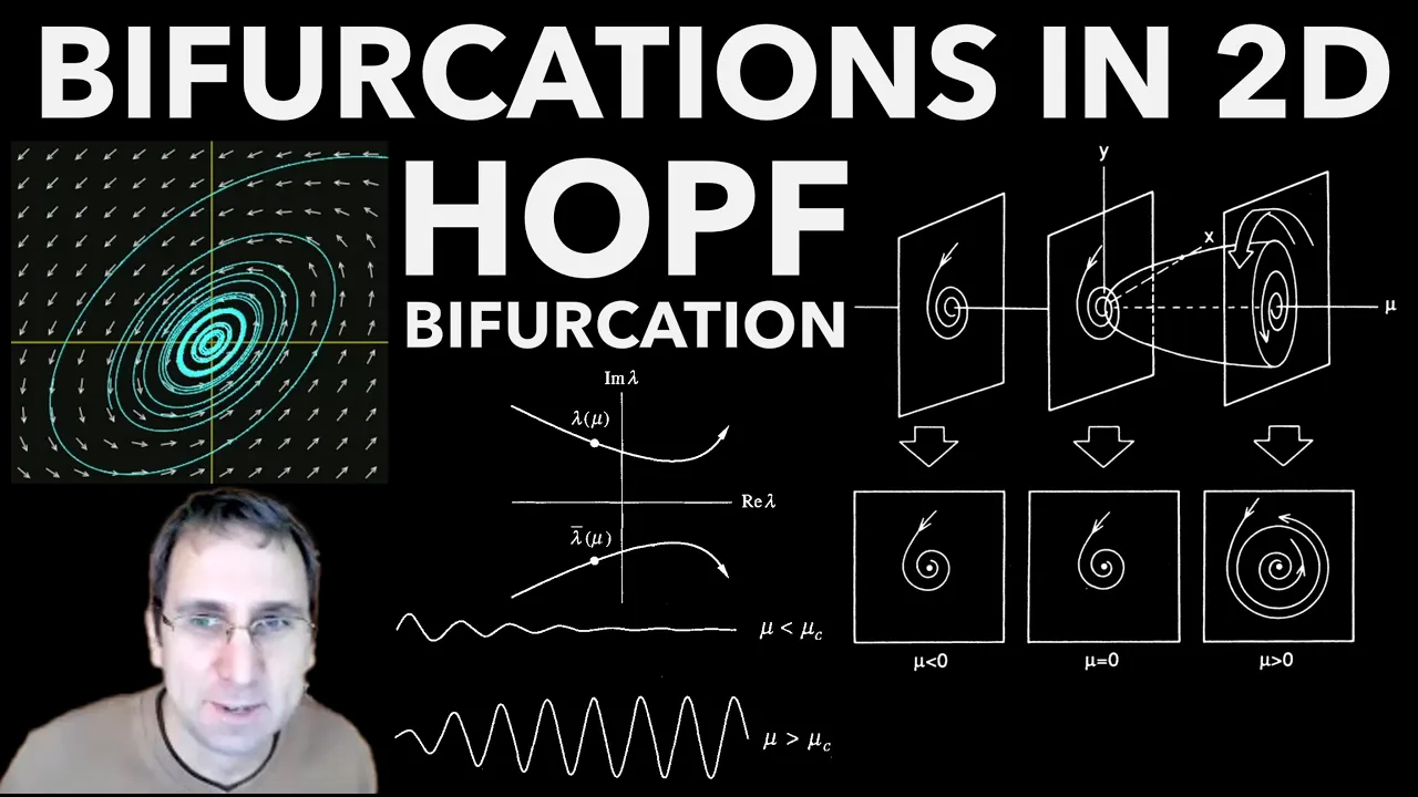








A limit cycle is an isolated closed trajectory in a dissipative dynamical system, representing periodic behavior that emerges through Hopf bifurcations when a stable critical point loses stability and gives rise to a stable limit cycle (supercritical Hopf bifurcation) or becomes unstable while producing an unstable limit cycle (subcritical Hopf bifurcation); unlike centers in conservative systems which have families of closed orbits, limit cycles are characterized by their isolation property and can only exist in dissipative systems where phase space volume is not preserved.
Limit Cycles in Nonlinear Dynamics: Hopf Bifurcations Explained
Added:Basic theory of Ordinary Differential Equations (ODEs), particularly coupled systems of first-order differential equations.
Phase space analysis, including understanding phase portraits, trajectories, and the classification of fixed points (e.g., nodes, saddles, spirals).
Linear stability analysis, specifically the calculation of the Jacobian matrix and the interpretation of its complex eigenvalues.
Introductory bifurcation theory, including one-dimensional bifurcations such as saddle-node, transcritical, and pitchfork bifurcations.
Distinguishing between Supercritical and Subcritical Hopf bifurcations, including the derivation of normal forms to determine limit cycle stability.
Global bifurcations in two dimensions, such as homoclinic and heteroclinic bifurcations, which describe how limit cycles are created or destroyed.
The Poincaré-Bendixson Theorem, which establishes mathematical criteria for the existence of limit cycles in two-dimensional plane systems.
Transition to chaos in three-dimensional systems, exploring strange attractors, Lorenz equations, and Poincaré maps.
Real-world applications of limit cycles in biological systems (e.g., the FitzHugh-Nagumo neuron model) and chemical oscillators (e.g., the Belousov-Zhabotinsky reaction).
30.6K views310likes39:56Original Release: 2014-07-28
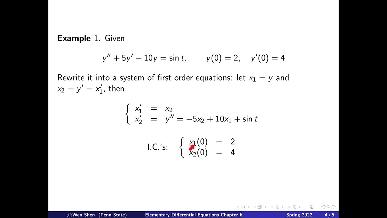
let's consider the possibility of critical points which are like lines now in some sense and i am going to do this with the help of an example let me look at a simple non-linear system where this happens again in 2 degrees of freedom 2 2 dimensions so let us look at x dot is equal to say mu x plus maybe a y plus x times x squared plus y squared and y dot equal to mu y so let us put an x here plus y with a mu where mu is a real parameter so this portion is a linear part of it and that is the non-linear part of it and it is immediately obvious from here that you have critical points you have a critical point certainly at 0 0 both these guys vanish and what sort of critical point is it if you linearize near the origin this l matrix is mu a 1 here minus 1 here and a mu here which implies that the trace is equal to twice mu and the determinant is equal to mu squared plus 1 in this fashion and remember that lambda 1 comma 2 is equal to minus t plus or minus square root of t squared minus 4 delta divided by 2 plus t so this is equal to twice mu plus or minus square root of ah t squared which is four mu squared minus mu square minus 1.
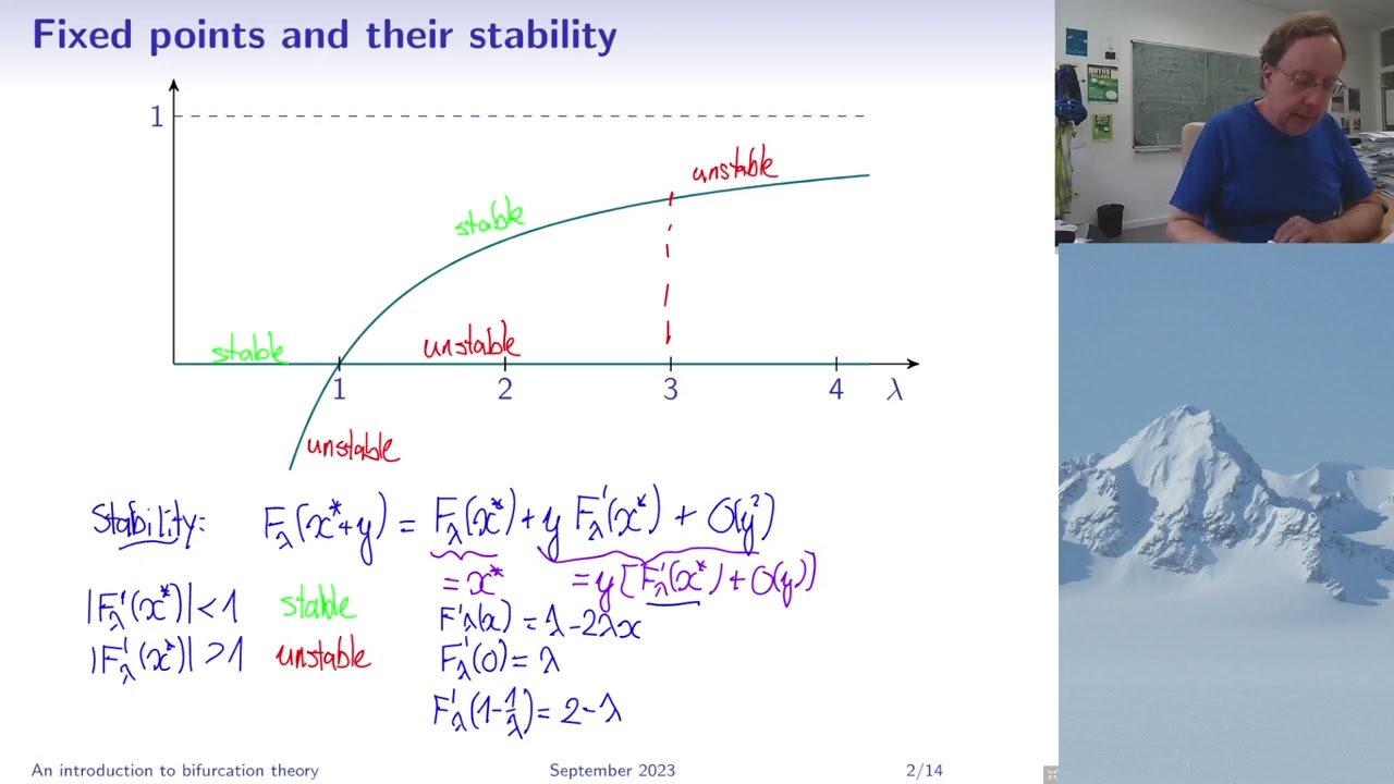
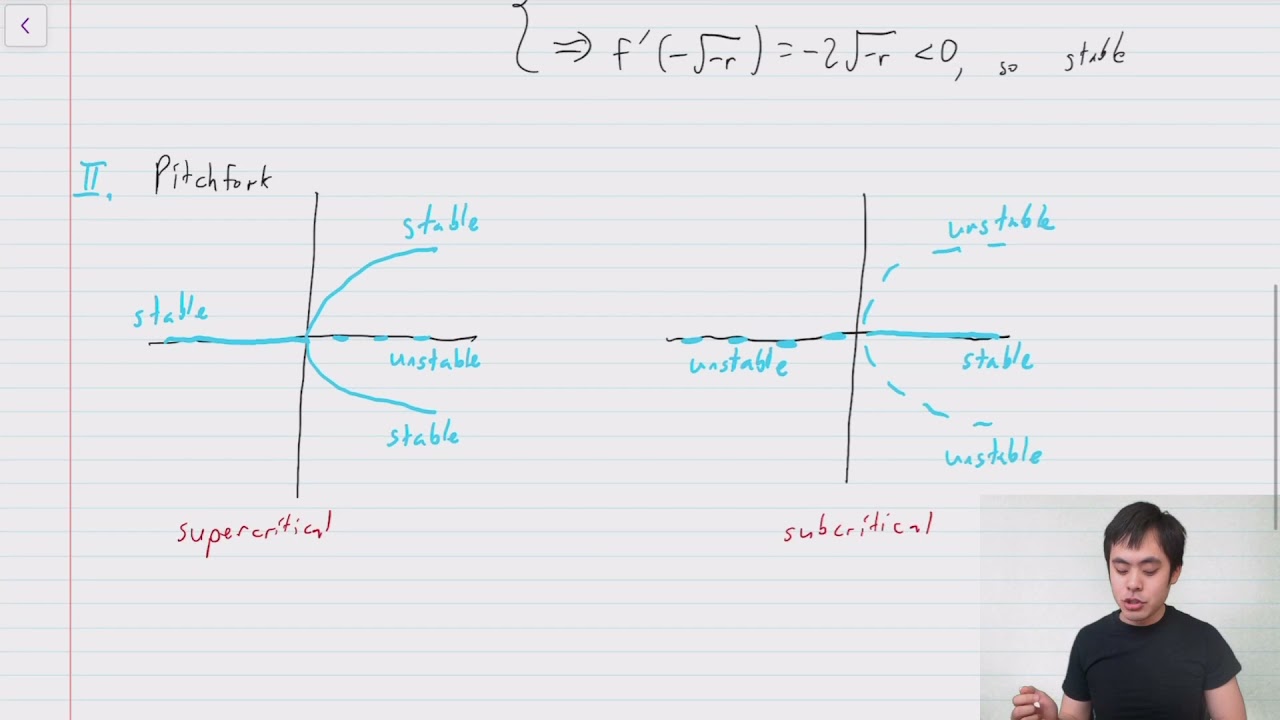
so it is 3 mu mu square squared four mu square minus four delta so that is four mu squared minus four divided by two so this cancels out here and this just gives you two 2i so mu plus or minus i so what kind of critical point is this depends on the sign of mu but since its complex conjugate as a pair of complex conjugate critical points its eigen values its clear that the critical point is a spiral point so this immediately says that it is an asymptotically stable spiral for mu less than zero and an unstable spiral for mu greater than zero at the origin and the phase picture as you can imagine is a spiral going inwards into the origin from mu less than zero and away from the origin outwards from u greater than zero we should like to know what the direction of the flow is as well for that let us go to polar coordinates plane polar coordinates so i said in the usual way x is equal to r cos theta y equal to r sin theta which immediately implies that r squared is x square plus y squared which implies if i differentiate both sides r r dot equal to x x dot plus y y dot and that becomes in the present instance i multiply this by x and this by y add the 2 and i get mu times x squared plus y squared so mu times r squared plus r to the power 4 which comes from these two terms and then this gets multiplied by x and this by y when you add the 2 it vanishes so this gives me r squared into mu plus r square in this fashion which implies that r dot is r times mu plus r squared therefore the picture which says that for mu less than zero this is an asymptotically stable spiral also shows that for mu less than zero there exists a trajectory corresponding to r equal to square root of minus mu on which there is no change of r at all and since r dot is zero the trajectory is a circle of some kind on the other hand if mu is positive this is an unstable spiral nothing happens everything flows off to infinity we would like to know the direction in which things flow and it is evident immediately that we have to draw two different phase portraits one for mu less than zero and the other for mu greater than zero so let us do that let us plot this for mu positive on this side and on this side for mu negative what kind of behavior do you have for mu negative for mu positive this is an unstable fixed point a critical point there on the other hand its stable so mu less than zero but it is also clear for mu less than 0 r dot equal to r times r squared minus modulus mu which is equal to 0 for r equal to square root of modulus mu therefore for mu less than zero there exists a circle of this kind on which you do not change r at all therefore this is a trajectory by itself on the other hand you have a asymptotically stable spiral here and outside here it is evident from this picture that if r is greater than square root of mod mu r dot is positive therefore the flow is outwards off to infinity on the other hand if r is less than square root of mod mu the flow is inwards r decreases towards the origin towards the stable fixed point at the origin the picture is very different for mu positive there when mu is positive this can never vanish so you do not have such a root at all such a solution at all and it is clear that r always increases the only question is in what direction do things happen and to find that we need to find out what theta does so let me write that down retaining this equation theta is tan inverse y over x which implies that theta dot is equal to 1 over 1 plus y squared over x squared multiplied by the derivative of this which is y dot over x minus y x dot over x squared and that simplifies to x y dot minus y x dot divided by x squared plus y squared if i go back to these equations of motion i multiply this by x and this by y and subtract if i multiply this by x i get minus x squared so let us write this down so in the present problem theta dot is equal to minus x squared minus plus mu x y plus x y times x square plus y square minus this is got to be multiplied by y and subtracted so minus mu x y minus y squared minus x y times x squared plus y squared that's the numerator and the whole thing is divided by x squared plus y squared it is immediately clear that these terms cancel out and you end up with is equal to minus 1 which means on that circle theta decreases at angular velocity equal to 1 in the clockwise direction because theta is decreasing so this means it does this on the circle therefore a point starting in the neighborhood of r equal to square root of mod mu this circle had a radius r equal to square root of minus mu what happens to a point in here it is clear that it is going to spiral in and fall into this fixed point asymptotically similarly it is evident that if i start a little bit outside i am going to spiral away towards infinity outwards that isolated closed orbit is called a limit cycle so let us define it this limit cycle and isolated limit cycle is an isolated closed trajectory and it's important to notice that it should be isolated in other words in its neighborhood there are no other closed trajectories there exists a neighborhood of this circle in which there are no other closed trajectories in this problem there isn't one in any case anywhere else except here notice on contrast that near a center if this were a center you would have a whole family of close trajectories of this kind arbitrarily close to this trajectory closed orbit there are other closed orbits and this is not a limit cycle on the other hand in this situation it is clear that this is a very special trajectory everything inside falls away from it everything outside falls outwards away from it therefore you would intuitively see that this is an unstable limit cycle you could have a situation where everything falls into it then it would be a stable limit cycle you could have a situation where things fall into it from one side but fall away from it on the other side of it and then it would be a semi stable limit cycle but the general situation is that a limit cycle is defined as an isolated closed trajectory it should be obvious immediately that you can't have a limit cycle in a conservative dynamical system because this means that whole sets of points are falling into this point here and whole sets of points are moving away there so there is no question of conservation of phase space volume here at all a limit cycle therefore a stable limit cycle is an attractor which occurs only in dissipative systems no possibility of limit cycles in a hamiltonian system in particular and in conservative dynamical systems in general we've defined conservative dynamical systems as those for which the phase space volume is preserved under the flow limit cycles therefore are a feature of dissipative systems in this instance the limit cycle was actually unstable but let's look at a slight modification we tweak this model a little bit till we get a stable limit cycle what would you need for that we'd like to have things go into it from both directions what would you require for that what should we do to this model we change things a little bit here so that we end up with stability there what would you suggest well had the situation been reversed namely had this become unstable and this becomes stable then the job would be done right all we need to do is to ensure that this becomes stable and this becomes unstable what should i do therefore find me minus mu okay we put a minus mu x then what put a minus here put a minus here would this do the trick well let's try let's try that's right what do you think happens well the linearized matrix near the origin is now minus mu a one here a minus one here and a minus mu here and the trace is equal to minus 2 mu the determinant is still mu squared plus 1 so lambda 1 comma 2 is equal to minus two mu plus or minus square root of four mu squared minus four mu square minus four so this becomes a two i so its just minus mu plus or minus i ok what next and what happens to the equation for r r dot what happens here for r r dot pardon me where should i put a minus x in the non-linear term i should put a minus sign here this is not going to work minus mu exactly i'm simply replacing mu by minus mu so do you think anything is going to happen maybe not okay so what's his suggestion what do you suggest what do you think i should do all of them should have negative signs this should remain as it is the non-linear term should have a negative sign okay we put a negative sign here and we put a minus sign there the linear the eigen values are not changed so let us draw this picture all possibilities can occur so let us draw what see what happens now it is evident here that these are the eigen values the way i've written it here because this not affected doesn't affect the linear terms and it says that when mu is positive you end up with a spiral which is stable and when mu is negative you end up with a spiral which is unstable right yes ok ok so let us go back to our original way of looking at it we had this and we change the sign here in which case this is mu and that's mu so we go back we do not change anything now it's this and it's this expression so this doesn't change it's an asymptotically stable spiral for mu negative and an unstable spiral from mu positive here but the equation for r r dot that definitely changes because this immediately says that r r dot is equal to multiply this by x multiply this by y and add the two and you get mu times r squared minus r to the power four in this fashion which implies that r dot is equal to i take out an r square and calc kill one of the r so you get r times mu minus r square in this fashion so once again we see there is a limit cycle and r is equal to square root of mu but this time for positive values of mu so what does the picture look like this one negative values of mu and this for positive values of mu now i have x as well as y so i really need to write down a proper bifurcation diagram but let us first draw what happens in the phase plane here is x here is y here is x and here is y and this corresponds to mu positive this corresponds to mu negative and for negative values of mu there is no root here r dot does not vanish anywhere other than r equal to zero and this is an asymptotically stable spiral and we should also check what theta dot does so let us do that theta dot is equal to x y dot minus y x dot divided by x squared plus y squared and i think it's not going to change so i multiply this by x i get minus x squared plus xy and i multiply this by y i get a mu x y and i put a minus sign so it is minus r square minus one the non-linear terms cancel out in any case so once again r mu is positive there exists a circle of radius square root of r equal to square root of mu this time on which the flow is in the counter clockwise direction and inside you have an unstable spiral point so it is evident that wherever you start other than r equal to 0 you are going to flow into this limit cycle if you start with a value of r bigger than square root of mu r dot is negative and therefore r shrinks inwards and therefore if you start here you are going to flow in into this point from outside on the other hand when mu is negative you just have an unstable spiral so this point is unstable here sorry you have a negative you have an asymptotically stable spiral and therefore wherever you start you are going to flow in this direction into the asymptotically stable spiral point it is quite clear that what has happened is that if you start from negative values of mu and move towards positive values what started off as a asymptotically stable critical point has bifurcated its become unstable but it is also given birth to a stable limit cycle something which is asymptotically stable and so the bifurcation diagram in this case looks like this i need to plot x and y equilibrium values so let us do that here and let us put this to be the mu axis and this is x and this is y i mean the steady state values the values on which things do not change at all then the only equilibrium point for mu less than zero is an asymptotically stable spiral point at x equal to zero y equal to zero so it is on this axis as soon as mu crosses over to positive values this point becomes unstable therefore in keeping with our usual notation we should really draw this with a dotted line like this and in its place you have a limit cycle which is stable of radius r equal to square root of mu but on the limit cycle x and y change without changing r and this radius of this limit cycle increases like the square root of mu therefore the picture would be something like this this really is a kind of parabolic ball which comes out whose size this radius here increases like the square root of mu and it is in both x and y you can see so its not a critical point its not an equilibrium point there is dynamics going on there but the moment you hit r equal to square root of mu it remains at that square root of mu and this is a stable limit cycle this is an unstable critical point and this was a stable asymptotically stable critical point and the bifurcation which happens at mu equal to 0 of a stable critical point into an unstable critical point and a stable limit cycle is called a hope bifurcation it is one of the most important bifurcations in non-linear dynamics happens all the time we will see examples of this when we study chemical and biological systems and oscillations in these systems this is a standard mechanism by which periodic behavior suddenly emerges from nowhere as you change your bifurcation parameter so on this thing you can see that it's a periodic orbit it's a periodic it's a close trajectory but an isolated closed trajectory because i have tailored this dynamical system to illustrate this point these were very simple functions here very specific functions and cancellations occurred therefore the limit cycle had the shape of a circle that's not necessarily true it could have a very complicated shape it could change there could be families of limit cycles but the basic definition of a limit cycle is that it is an isolated periodic trajectory in a dissipative system and discovering limit cycles is not anywhere near as easy as finding the fixed points or the critical points of the system for which all you have to do is to equate the right hand sides to zero in some sense but this is not so for limit cycles especially if you don't if you are not able to reduce things to very simple things simple algebra using say polar coordinates or anything like that so the shape of the limit cycle is complicated you can only discover this numerically but there are theorems and criteria which will tell you when these limit cycles could exist and whether such limit cycles could exist incidentally from this picture it is also clear that inside this stable limit cycle there must exist at least one unstable critical point otherwise there is no way these things would get thrown out and move into this limit cycle here and that is measured by something called the the winding number or the poncary index which i will come to a little later yes can i oh yes why not yes open trajectories we are not considering here at all because they are not of much interest to us at the moment but close trajectories would mean periodic motion and we'd like to start with things which are periodic and maybe apply perturbations and go to things which become quasi periodic or aperiodic this is going to be the thrust of what we are doing open trajectory is unbounded motion in general is not of direct interest there are of course many physical situations where it is important but they are not directly of concern to us here specifically we are always looking for periodic motion or things close to periodic motion in some fashion the earlier example what happened in the earlier example if i put a plus sign here what happens now what kind of behavior do you have once again since we have chosen this mu to be exactly as it is this is certainly true you have an asymptotically stable spiral from mu less than zero and an unstable spiral from u greater than zero but because we change the sign of the non-linear term this becomes a plus here it becomes a plus here in this case and then the picture gets reversed this is for mu less than 0 and this is for mu greater than 0 for mu greater than 0 this was an unstable spiral here so this is unstable and things are going to go flow away from it certainly for mu less than 0 this is a stable spiral point asymptotically stable spiral point things are going to flow into it but this trajectory here at r squared equal to square root of minus mu is certainly going to be an isolated trajectory here but i should really draw it as a dotted line because it is unstable and it is evident that here things are flowing away in this fashion on the other hand here things are going to flow into this origin this is stable so it is going to flow in here and things are going to flow starting here flow outwards this is therefore an unstable limit cycle and it contains within it a stable critical point so here what's happening is as you move from positive mu towards negative mu what was an unstable critical point has bifurcated into a stable critical point and an unstable limit cycle so if you like its the image it is the complement of what happened earlier and let us draw the bifurcation diagram in this case and you have a picture where as a function of mu so here is x here is y and here is mu for mu greater than 0 you had an unstable critical point therefore it was like this in this case and it becomes stable for mu less than zero so this is unstable and this is a stables critical point asymptotically stable critical point however you have now a limit cycle that is unstable and therefore i should really draw it with a dotted line like this and these are the trajectories on it and this is an unstable limit cycle compare this with the earlier case where you had it does not matter which way this parabola looks the way we have written and drawn it this is move to the right here but it is not necessary this was stable and inside it you had an unstable critical point and this was a stable critical point so a stable critical point came along bifurcated into an unstable critical point and a stable limit cycle and this was a stable critical point and this was an unstable and this is what we call a hope bifurcation this two is a hope bifurcation this is called a sub critical and this is called a super critical of bifurcation in either case it's the bifurcation by which a critical point bifurcates into a critical point and a limit cycle and the stabilities in the two cases are as i have shown here the fact that this parabola looks to the right and that looks to the left is an artifact of the way we have drawn this with the way we have chosen coefficients but the essential point is that a stable one a stable critical point bifurcates to a stable limit cycle here and loses its stability in a subcritical bifurcation on the other hand an unstable critical point gains stability but also gives rise to an unstable limit cycle in the process both these processes happen very often in nature but as i repeated i said earlier they happen only in dissipative systems you have limit cycles only in dissipative systems here is a simple example of a system with limit cycles so let us consider r dot equal to sine pi r and let us say theta dot is equal to 1 in polar coordinates so i have already gone to polar coordinates and done this what would you say is the behavior of this system what does it do in polar coordinates if it does this then we could go back and write the equations in x and x dot if you like but we can analyze it directly as it stands here what would you say is the behavior of the system on the right hand side when does the right hand side vanish in the first equation so it is evident that limit cycles at r is equal to 1 2 3 and so on we do not yet know what is happening at r equal to 0 which is the origin and you have presumably a critical point at that place we do not know the nature of this critical point what kind of limit cycles do you have at various places would it be stable or unstable or what how would you decide this yes you're quite right they would alternate in stability one would be stable the next would be unstable and so on what would be the one at r equal to one for instance sine pi r near r equal to one you have to do a taylor expansion about r equal to one and of course sine pi is zero so the first term is 0 plus the next term is r minus 1 times the derivative of sine pi r evaluated at r equal to 1 and what is that it is pi cos pi r right so there is a pi cos pi r at r equal to one so that is a cos pi and this is equal to one minus r in the vicinity of r equal to one plus higher order terms so it is really telling you that r dot is of the order is of the form one minus r is this therefore a stable or an unstable limit cycle at r equal to one if r is less than one it's growing and if r is greater than one is shrinking therefore it's a stable limit cycle so we immediately realize that at r equal to one you have a stable limit cycle it is not hard to see at r equal to two you get a cos two pi here and that would become plus one and therefore it would become unstable therefore the picture in this case would look like this at r equal to 1 you have a stable limit cycle at r equal to 2 you have an unstable limit cycle at r equal to three you have a stable limit cycle once again this corresponds to r what would you therefore expect is the behavior at the origin which is a critical point it should be unstable so that things would flow into it and i would therefore expect that in this case everything goes around the counter clockwise direction therefore i would expect trajectories to do this so all points between r equal to 2 and r equal to 1 1 would eventually fall into this trajectory they would fall into this stable limit cycle what is the basin of attraction of the limit cycle at r equal to one so we have the concept of the basin of attraction of the stable limit cycle r equal to one is all points which lie inside they are going to move outwards except the origin which is a critical point by itself so you really have an unstable critical point there so this is 0 less than r less than 1 and what happens to points between 2 and this a 2 fall in so in fact less than two points on r equal to one are already there at this point and similarly for the basin of attraction for this is everything between two and less than four would fall into this and so on so this is the second kind of attractor other than a critical point point attractors we now have closed orbits as attractors and you can easily see that one could generalize this and have in higher dimensions you could have a torus attractor you could have an n dimensional torus as an attractor but the interesting thing and we will see this a little later is that for high dimensions dimensions greater than 2 you have another kind of attractor possible called a strange attractor and those could be very complicated fractal objects and they would be the ones of central interest to us as we go along in real non-linear systems so i stop here today and then we take it up from this point we have seen some of the elementary bifurcations here and we will see what other possibilities can exist for dynamical systems of this guy no they needn't the question is can limit cycles do limit cycles have to be circles the answer is no of course not it happened to be they happen to be circles in the examples i showed because i have contrived it in that fashion i've written this already in polar coordinates in a simple way and in the earlier example i had very simple functions of r squared but there is no reason why they should be so at all the very first example of a limit cycle which occurred was in triode oscillations and its called the wonder pole oscillator and it has a term which goes like its again a two dimensional dynamical system there is an x double dot term which would be the inertia term plus a term which is proportional to x so some natural frequency square times x plus a damping term and if it is a simple harmonic damped simple harmonic oscillator linear oscillator this would be a constant times x dot but you have here a term which looks like 1 minus x square times x dot times some coefficient and this equal to 0 is a non-linear equation because of the presence of this term x squared x dot and you can see that this damping for x squared less than one acts like normal damping but x square greater than one it feeds back into the system or if you like you put a minus sign here this would reverse the situation and say for sufficiently small x things would tend to grow outwards and for larger x they would tend to come back this direction so the damping acts in a state dependent manner its dependent on x so either you have positive feedback or you have negative feedback depending on what x itself is and the limit cycles of this system were the first limit cycles to be discovered and this is the wander pole oscillator i am not too sure about the signs here but this is essentially what it is you could change this constant it does not matter but this is the way this system behaves and as i said earlier this occurred for the first time in the consideration of triode oscillations in a triode the old vacuum tube so we will see further examples of limit cycles bye
Up Next
18:39
The Logistic Map: Unlocking the Universal Chaos in Nature and Mathematics
@veritasium
16.8M views•2020-01-29

4:43
Elliptic Curve Cryptography Explained: ECC, ECDSA, ECDH
@PracticalNetworking
28.5K views•2024-10-21

50:04
Uncountable Sets & Cardinal Numbers in Real Analysis
@iit
51.9K views•2016-01-19

6:00
The Mathematical Impossibility of Accurate World Maps
@Vox
23.3M views•2016-12-02
Related Study Plans & Knowledge Roadmaps
Structured learning paths in Mathematics
mathematics
Tensor Calculus: Vectors to Riemann Curvature
01Mathematical Foundations: Linear Algebra & Calculus
02Covectors, Dual Spaces, and Tensor Basics
03The Metric Tensor and Index Gymnastics
+ 2 more learning modules
40h5 modules
Explore Roadmap
mathematics
Gödel's Incompleteness: Logic, Proofs & Limits
01Introduction to Formal Systems & Hilbert's Dream
02Set Theory, Cardinality, and Cantor's Diagonal Argument
03Arithmetization and Gödel Numbering
+ 2 more learning modules
14h5 modules
Explore Roadmap
mathematics
Galois Theory: Fields, Groups & Solvability
01Foundations of Abstract Algebra: Groups & Fields
02Polynomials & Field Extensions
03Splitting Fields & Symmetries
+ 2 more learning modules
24h5 modules
Explore Roadmap
mathematics
Non-Euclidean Geometry: Models & Geodesics
01Euclid's Fifth Postulate and the Birth of New Geometries
02Hyperbolic Space and the Poincaré Disk Model
03Geodesics: Defining Straight Lines in Curved Spaces
+ 2 more learning modules
15h5 modules
Explore Roadmap