




![[이얼 대학수학] 정필권 경제수학(Mathematical Economics) 제97강 제4부 미분방정식과 정차방정식 22.7절 2변수 위상도](https://i.ytimg.com/vi/hLm_jxXcN4E/maxresdefault.jpg)


![Бифуркации векторных полей на плоскости [4] // Наталия Гончарук](https://i.ytimg.com/vi/achZNQKLes8/maxresdefault.jpg)



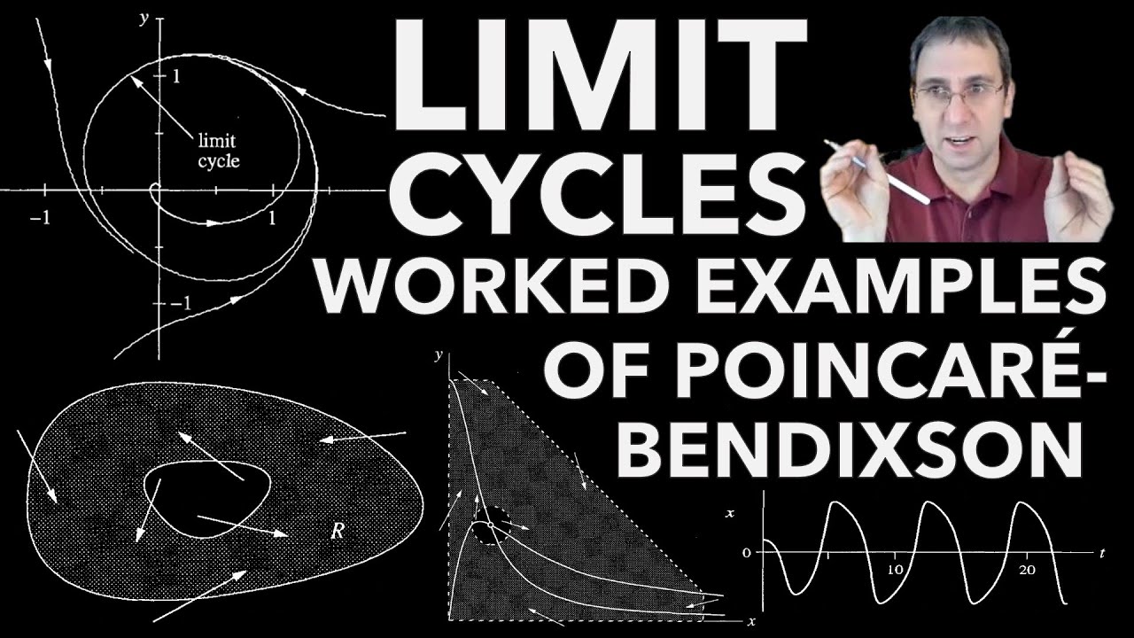


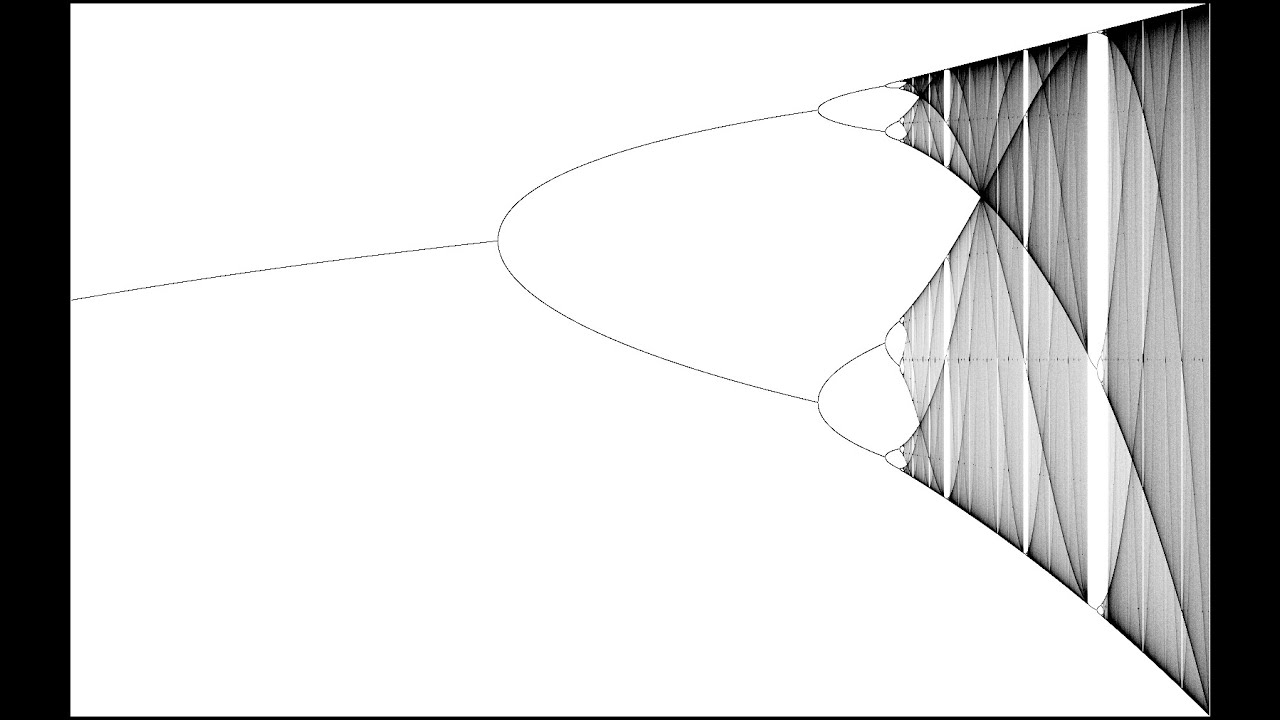



In two-dimensional dynamical systems, bifurcations of fixed points occur when eigenvalues cross critical boundaries, with three main types: saddle-node bifurcations (where a saddle and node collide and annihilate), transcritical bifurcations (where stable and unstable fixed points exchange stability), and pitchfork bifurcations (which can be supercritical or subcritical, creating or destroying symmetric pairs of fixed points); additionally, Hopf bifurcations represent a qualitatively new phenomenon where complex conjugate eigenvalues cross the imaginary axis, leading to the creation or destruction of closed orbits (limit cycles), with the amplitude of the limit cycle scaling as the square root of the distance from the bifurcation point.
Bifurcations in 2D Systems: Fixed Points & Hopf | MAE5790-12
Added:Fundamentals of 1D dynamical systems, including phase lines, fixed points, and basic bifurcations (saddle-node, transcritical, and pitchfork).
Linear stability analysis in 2D systems, specifically using the Jacobian matrix, eigenvalues, and eigenvectors to classify fixed points (e.g., nodes, saddles, spirals).
Phase plane analysis, including plotting vector fields, trajectories, and identifying nullclines.
Basic understanding of ordinary differential equations (ODEs) and coupled systems of differential equations.
Global bifurcations in 2D systems, such as homoclinic and heteroclinic bifurcations, where limit cycles interact with saddle points.
The Poincaré-Bendixson Theorem and its application in proving the existence or non-existence of limit cycles in 2D phase space.
Transition to chaos and higher-dimensional systems (3D+), exploring concepts like strange attractors, the Lorenz equations, and period-doubling.
Real-world biological and chemical oscillators, such as the FitzHugh-Nagumo model for neuron firing or the Belousov-Zhabotinsky reaction.
55.4K views419likes46:54Original Release: 2014-05-27
Well, I have corrected your tests and so um I want to leave something like a half hour at the end of the class to talk about the test also to return them.
There's a lot of uncollected homework too. Um homework three and four, homework one.
So we have a lot of logistical stuff to deal with at the end. But um before we do that, let me begin a little bit of chapter 8, which is we're now moving into the logical next step of the course, I guess you could say. That is, if you think about it, we started with one-dimensional systems, looked at what dynamics could occur on the line and then classified various kinds of bifurcations that could occur in one-dimensional systems. After that we moved to two-dimensional systems. Saw that in addition to the fixed points that we could have in 1D. Um we could also have a new type of thing which are closed orbits representing periodic motions. And we also had more exotic stuff like homocinic orbits. Uh anyway, but the time has come to look again at bifurcations but now in two-dimensional systems. And so that's chapter eight.
So let's suppose that we've got a um there exists either a stable equilibrium point that is a fixed point or a uh a closed orbit. Those being the two main types of phenomena that we've been interested in.
So our questions as before would be how can those things vanish? How could they change stability as we vary some parameter? How can it vanish or change stability as we vary a parameter?
And so today uh I'd like to just mention a few very simple cases which are normal forms that is sort of the simplest model differential equations that can show some of the phenomena we're interested in and then in later lectures we'll talk about some scientific examples of these.
So today protottypical examples of such bifurcations. Technically these are related to the idea of normal forms which you can learn about in more advanced courses but um I'm not really saying carefully what normal forms are.
You know, roughly speaking, it means that through a suitable change of coordinates, you can reduce a system showing one of the bifurcations that we're going to discuss to one of these normal forms. All right.
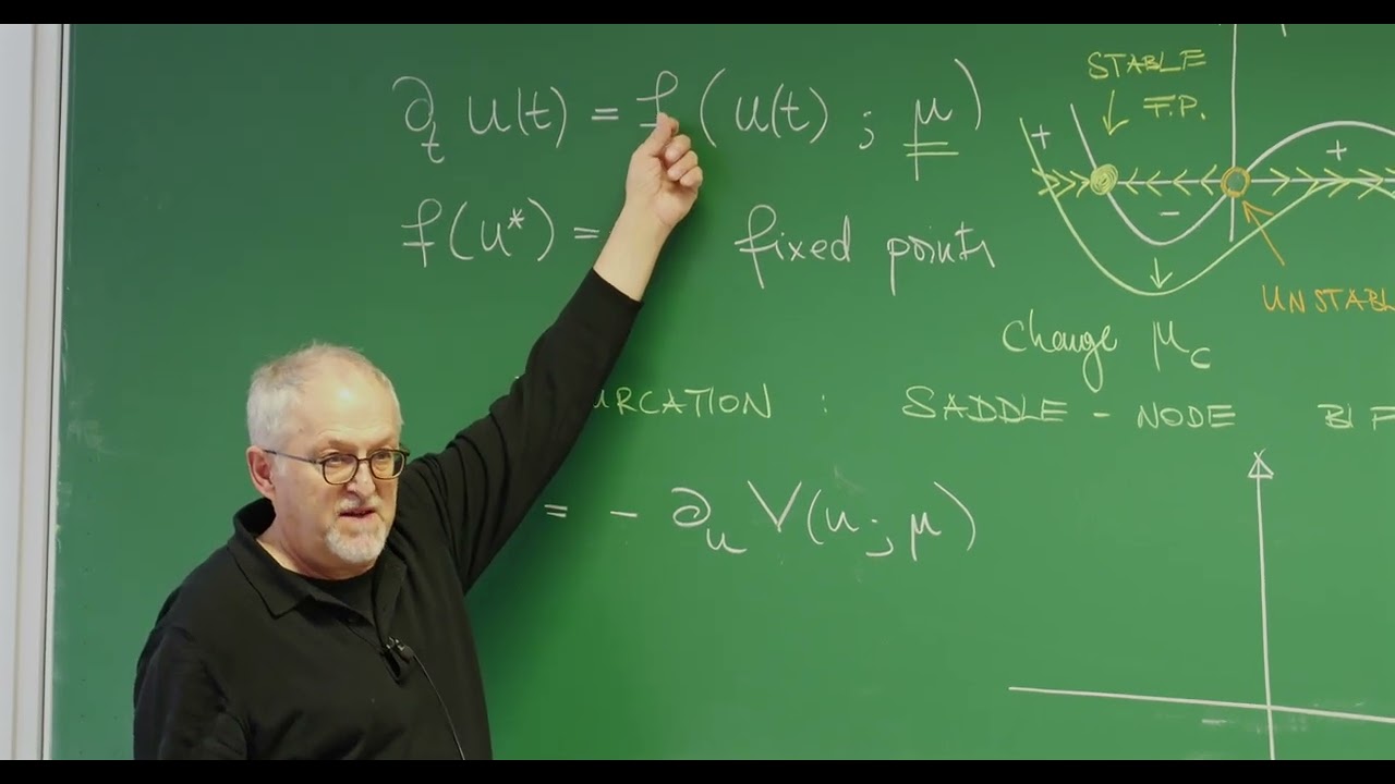
Um so first let's talk about bifurcations of fixed points and um those can be divided into two main types. We've got bifurcations that occur when some igen value equals zero. And these come in three main flavors which we've already seen. Saddle node, transcritical and pitchfork. And as we've seen them in our one-dimensional systems, well, not very much different happens in two dimensions. Uh except that the term saddle node will start to make sense in two dimensions in a way that it didn't in one. But the really new thing that can happen is that we can get a uh a bifurcation where a pair of igen values that are complex conjugate become pure imaginary. So lambda equals something of the form plus or minus i * a real number omega. And this is an example of or I mean this will lead to what we call a hop bifurcation named after one of the mathematicians who studied it although he really wasn't the first. Plankare had seen them too back in the early days of the subject but anyway everyone calls these hop bifurcations and they um are really something qualitatively new for us. They lead to the creation of closed orbits.
So you might wonder why are we talking so much about the igen values. So let's just remind ourselves that the importance of thinking about the igen values at the fixed point if we have both real parts that is the real part of lambda 1 and lambda 2 and of course we have two igen values we're in a two-dimensional system here. If the real part of both of those are negative then the fixed point will be stable locally. That is the fixed point is linearly stable because the real parts control the decay rate the exponential decay rate of the solutions near a fixed point. So um it's convenient to draw a little picture where we look at where the igen values are in the complex plane as we change a parameter. That is if we make a graph with imaginary lambda on this axis real part of lambda here.
Um then the two kinds of things that we can have two types of situations for a stable fixed point are you could have both lambdas negative and real like this or um since we're studying problems with that are real vector fields the the characteristic equation for the igen values is going to have real coefficients and it'll be a quadratic equation because we're in a two-dimensional system. So the lambdas will always be complex conjugates or they'll both be real. And so the other case is that you could have um a complex conjugate pair like that. Uh and so we have to think then what can happen? How can we make these get um into the unstable half plane?
That is the half plane where the real part of lambda is positive.
That's what will lead to a bifurcation. Bifurcation occurs when the igen values cross into the right half plane um the plane where the real part of lambda is greater than zero. actually it occurs when you know when it's equal to zero. So um the other thing though before we get into the details of this case one maybe I'll just say what's about to come is that there's also bifurcations of periodic orbits closed orbits whatever you want to call them. Um and so you could say in a way we've already talked about one this hop bifurcation involves periodic orbits but but it can be thought about by just thinking about a fixed point. So in a sense it's easier than these other cases that we're going to talk about later which are um you can have coalescence of cycles that is you could imagine something analogous to the saddle node bifurcation of fixed points where a stable and an unstable one come together and annihilate. You could have that with cycles too. You could have a you know a stable cycle outside of an unstable cycle say and then as you change a parameter they come closer and closer together and eventually merge and then disappear. They coalesce and disappear that way. So that'll be one kind of phenomenon sometimes called saddle node bifurcation of cycles or another that we can have goes by various names. Um some people call it a sniper, some call it a snick. Um so this would be saddle node infinite period bifurcation where you can see there there's s n i p eer saddle node infinite period. So that's another interesting mechanism.
This would be saddle node on an invariant circle. It's the same bifurcation. And that's an interesting picture where you have a closed orbit that um is stable, but then it suddenly as you change a parameter develops one of these funky halfstable points. Kind of half stable. if it were just a one-dimensional system and then that thing can split into a saddle and a node on the cycle where there's a stable point there and everything's being attracted on the cycle to that. Um so you can see what I mean saddle node on this invariant circle meaning just this closed loop. So if you picture it going this way, as these two points come together and collide and then annihilate, you'll be left with a uh a cycle where the flow is just going around like that. There's also stuff happening on the inside which we haven't talked about yet, but you know, I mean, the flow can come out towards those points. So you can see this is a a saddle here. That's a node. Anyway, we'll go into detail about this later.
So that's another interesting bifurcation on a that can destroy a periodic orbit. By the way, why do I say infinite period maybe you can visualize it that as you're coming around here if a fixed point is about to be born things are going to be very slow near this point even though you get through there you kind of go takes a long time to get through and then you go around. So right at the bifurcation it will take infinitely long to go around the loop. Whereas in this picture there's no change in the frequency at the bifurcation. You're just going around comfortably. Anyway that's one third a second case the sniper coalescence. The third is a thing called a homoc clinicinic bifurcation which um I don't think I'll attempt to draw here but we'll get into it later. It comes up when we're thinking about a forced pendulum problem. That's one nice example of it.
So anyway, that's to come. But but for the rest of this lecture, let me just touch on some simple examples of the um bifurcations of fixed points. Is there any comment or question at this stage?
Okay. All right. So let's go back to our case one of fixed points and I'll just touch on this kind of lightly that is these lambda equals zero bifurcations zero value bifurcations are um so similar to what we've already done that I hesitate to even say anything about them but let's just talk about them briefly. Okay, so the saddle node in two dimensions would look here's a a very simple example of such a system. You could take x dot= a minus x^2 and um y dot is - y sorry not negative lambda y let's just say negative y. So you know the x and the y are decoupled there. It's just two kind of two separate one-dimensional systems doing their own thing. And you can notice nothing interesting is happening in the y direction. Everything is just damping out exponentially to y equals z pushing you onto the x-axis where the relatively interesting stuff is happening as you vary a. So the moderately interesting dynamics are occurring in the x direction.
and um just having damping in the other direction. So if we wanted to analyze this uh well of course there's fixed points when a is positive they would be square<unk> of a comma 0 and minus square<unk> of a comma 0. When a is greater than zero and then as a approaches zero those fixed points come closer together and eventually annihilate when a equals z or coales then annihilate for at negative a.
uh so if we look at the Jacobian at each of those fixed points well we'll get Jacobian matrix A. So it's dx dot or partial x dot partial x partial x dot partial y partial y dot partial x partial y dot partial y gives us uh -2 x we're evaluating it at a fixed point. So x star 0 01 and so you can see that the well it's diagonal matrix so the lambdas are just lambda 1 is min - 2xar and lambda 2 is not going anywhere that's just stuck at -1. Notice that um the case that corresponds to a stable point is the one where this lambda is negative. This one's already negative in the left half plane. But if x is a negative number that is um sorry if x is a positive number because I have that negative sign. So if xar equals square<unk> of a yar= z this is a stable node.
Whereas the other point minus square<unk> of a 0 is the saddle. So this is why we're talking about saddle node bifurcation. I mean it is now finally revealed because in two dimensions or higher the thing that's the two points that are colliding are a saddle and a node at such a bifurcation.
Um and so if we look at the uh igen value picture that is the spectrum where we look at real lambda and imaginary lambda as a function of a we have one value sitting here at minus1 and the other is at negative uh<unk> 2 * a sorry -2 * the<unk> of Okay. So notice that as we change the parameter a towards zero, what's happening is that this igen value is not moving. In a less contrived example than this super simple one, this igen value might move a little bit as you change a but um not much. The dramatic thing is this igen value which is rocketing towards zero.
I shouldn't draw an arrow because it's not a phase portrait, but you know what I mean. As I turn the knob on a, this point is moving towards zero. And so that's why we speak of a zero igon value bifurcation. This value will actually cross through zero at the bifurcation or not cross through I mean it will hit zero and then when lambda is negative we don't even have these fixed points anymore. So we can't speak about it going through but it will go to zero and then poof the bifurcation has occurred. So um if we were to draw the phase portrait that corresponds to this picture maybe we should do that. Then in the xy plane we say we have um a fixed point at a square root of a z. So over here and then another one over here.
uh and we decided that the one on the negative side is a saddle. Actually you can see that there are invariant lines here when x is equal to square<unk> of a or negative<unk> of a we have these invariant lines. So and and actually the flow on those lines is just exponentially damped you know decay down to these points. So that's easy getting that. If you look on the y axis, is anything special happening? Not really. Um x dot is positive there. No, negative for this case. So it looks like we would be wait, have I done that right? Um if uh I'm doing the case where Oh, I see. because I'd be looking at x equals z. I'm talking about a positive, right? So, I'd be flowing to the right like this and over here we do that. So, this is a stable point. That's a stable node as advertised. And this really is a saddle. Also, the x-axis is invariant, so easy to see what's happening on there. But I mean, this picture sort of gives you a hint of why did we study one-dimensional systems for so long? You might say that was kind of trivial. Why did we spend all that time on that? And this picture is kind of the justification that that when you're doing bifurcation theory, what tends to happen is that the flow trans that there's interesting dynamics in one dimension that kind of dominates everything. In this case, it's the x-axis and the other dimensions um lead to just kind of boring collapsing behavior like we're seeing here. So in the long run, everything is controlled by what happens on this one-dimensional manifold, which here is just the x-axis. But in general, we'll see in other problems, there might be some curvy one-dimensional manifold, but there's sort of these stable and unstable points moving along that manifold, like beads sliding on a necklace and then banging into each other. So, this is giving a representative picture of what we'll see in more complicated settings. Um, then at a equals z, these two points come together and merge.
Let's look at that curious picture. Maybe I'll do it over here. So this is the a positive picture both of these.
Um actually let's make some more room.
[Music] So a equals zero we get this strange looking picture uh as far as the real lambda imaginary lambda plane goes We now just have still have our igen value sitting at negative one and the other has gone into zero and that's when the bifurcation occurs back in the phase plane we have if you kind of imagine smooshing these two lines the vertical lines here that invariant line with this one. As those come together, what are we going to see? Uh, you'll see a picture that looks sort of like this kind of funny hybrid fix point there at the collision with stuff flowing in from this side and flowing out from this side. All right. Right? Does that seem plausible as the the limiting picture by pushing those two lines together? I probably shouldn't show this as a half-filled circle because it's not really half stable. If you think about it, it's got well, it is in a way. I mean, it attracts half the picture, right? The whole right half plane is getting attracted to this point, whereas the whole left half plane is running away from the point. So, maybe that's okay. I was thinking in terms of directions. It has three incoming directions along invariant lines but only one outgoing. So feels like in a way it should be threequarters stable but that's not really I don't know whatever it's a nonsense thing to worry about how you draw the dot. It's it's partially stable and partially unstable.
Okay. So and then for a negative um the fixed point doesn't exist. So you can't draw the spectrum at the fixed point because there is no fixed point.
Um but instead you would have over here in the phase plane a picture that is kind of confusing.
There's this slow region here that's amorphous. I don't mean to indicate a cloud really just that there's a kind of slow patch where trajectories will come in there and then you could even think of it I mean in other in certain places in the book I refer to what's left over after this point disappears as a ghost that is there's nothing there but there's a kind of a ghost of the former fix point which has the effect that when trajectories enter the ghost region they go very slowly even though there are no fixed points there because the vector field is close to zero in magnitude. So you go slow through there then kind of come out and then you're fast again on this side. So sometimes you'll see dynamical systems that get hung up in some region they do get through. It's also sometimes called a bottleneck.
where the flow goes slowly through that as if there were a constriction there like in a bottle anyway. Okay. So that's a typical scenario for saddle node in two dimensions. Any question about that? So all right. Um I think I will leave the transcritical case to you. You can see this is pretty easy to do these analyses.
Um if you want to look at it, it would be the model system would be x dot is ax - x^2 y dot is minus y. So you analyze it in the way that we just did. And the third case is pitchfork.
And as you may remember with the pitchfork, there are these two flavors.
There's a subcritical and a supercritical. We'll be talking a lot about that. It actually comes back in in the case of hop bifurcation too that there's sub and superc critical and I'll try in the next lecture actually sort of a high point don't skip the next lecture because I'll be showing some movies. So I'll show movies of real things undergoing bifurcations like airplane wings undergoing aerolastic flutter or um chemical oscillations. So and then we'll talk about you know what kind of bifurcation is that just from watching the experiment so that you get some intuition about that these are really meaningful things not just math I mean meaningful in the real world obviously math is more meaningful than reality no we're all Pythagoreans here so let me show you the superc critical version of the pitchfork we'd have um this as a a model for a normal form. X dot is ax - x cubed. Y dot is again something boring - y. Uh and you know in this picture drawing again our our various both spectra and phase portraits.
Um well the spectrum if you calculate the fixed points here we've got um the vector xar is say square root of a plus or minus comma zero.
And um there's also a fixed point at the origin. So three fixed points if a is positive. And so if I draw actually I seem to be drawing the case a negative first. So in that case these this pair of fixed points doesn't exist and all we have is just a stable point at the origin. So there's a node and you can check that the flow looks like this and maybe say like that as a gets close to zero. So we're just coming in um the igen values at the stable point that is the igen values at the origin which is stable when a is negative are just you can check to be -1 and a negative yeah no just a so this is at the origin We're looking at the Jacobian there. The maybe I should just say the Jacobian would be a 0 01. The a being just from this term ax and the negative 1 from this term negative y. Okay. So anyway there's the jacobian. And then as we change our parameter a again moving it towards zero. This point marches towards zero hits zero. Now when it hits zero that means that these two fixed points are about to be born.
So when a is zero we get a um diagram that looks like this in the phase plane still coming in on this direction. This point is still stable but we almost move vertically and then very slowly come in kind of sideways like this. That is the trajectories are really they go to zero very slowly because you can see it's going to be behaving like x dot is minus x cubed the a is missing a is zero and this has a very slow decay only algebraically fast not exponentially fast.
So the physicists refer to this as critical slowing down that occurs at this transition and it's real. It can be seen in experiments in second order phase transitions. Um and then so back over here in the lambda plane we would have one value at negative 1 and the other at zero. Okay. Now finally when a is positive then our picture in the phase portrait would be like this. We have these invariant lines again. Now there's a symmetrical pair of them. They go through these points and the origin then becomes a saddle. We flow this way towards these stable points. And likewise over here. So that's the superc critical pitchfork. We have split out of this stable point. It just burped out two new stable points on either side symmetrical pair here and here and became a saddle. And we call it super critical because these newly created fix points are stable.
So it means the new branch of fixed points that is um they're actually branches uh with xstar equals plus or minus<unk> a stable.
Okay, any question about that? I mean, I guess it's pretty much what you would have expected knowing what we know about one dimension. All right, so let me um throw in a little bit about the hops bifurcation, then we'll stop and discuss the test. But okay. So um let's talk now about the hops case. So lambda is plus or minus i omega. I'm writing omega because it really does represent a frequency. This imaginary it'll in fact be the frequency of the limit cycle at birth.
So an equivalent condition for this is to have a pure a set of pure imaginary igen values is this is what we were seeing. You know all the times that we thought we had a center we weren't sure if it was a center in a nonlinear system. If you just ask does this system have a linear center that's the condition for a hop bifurcation. That is you look for places where the trace is zero and the determinant is positive. We did a problem about um a a model of glycolysis you may remember where we were um looking for the it was back in the days of doing the plank ben Dixon theorem. We constructed that strange trapping region remember that looked like this.
And we asked for this point in the middle to become unstable. That that point was undergoing a hop bifurcation.
We just didn't know it back then when we created the limit cycle. So anyway, what is the um let's talk about the case of the superc critical hops and then in the next lecture I'll discuss the subcritical case and that's when we'll watch movies of the various types.
Anyway, in the superc critical case, what happens is that a stable spiral lives on one side of the bifurcation and as you cross through the bifurcation, you can cross it in either direction, but let's suppose we turn a knob and we go from I've been sort of assuming we always start with a stable fixed point like you have a system at equilibrium that then loses stability. And so as we turn our knob, the uh stable spiral point is going to bifurcate into an unstable spiral. But it's not just by itself anymore. The unstable spiral will be surrounded by a small amplitude limit cycle.
there'll be a little tiny baby limit cycle around it and it always has an elliptical shape um at least near birth and it'll be stable small amplitude stable nearly elliptical limit cycle.
And under pretty generic conditions, this really will be a limit cycle. I don't have to say closed orbit like I'm usually careful to do. It'll really be isolated. It'll just be a So this is there's a thing called the hop theorem, which is a nice theorem for guaranteeing existence of a limit cycle that is um stable in this case. In the subcritical case it will be unstable. Anyway, so this is it. Now let's just look at a picture of what that would be.
Oh, I suppose maybe I should also say something about the igen values because we were talking about them. So at the bifurcation the lambdas will be plus or minus i omega as mentioned and um so if we want to see this an example would be suppose we do it in polar coordinates r dot equals a r - r cubed and theta dot is omega And then it turns out in the theory of normal forms you can show that near a hop bifurcation this is what the dynamics will look like typically that that the frequency of the rotation will have some constant term but it'll also depend on amplitude generally through the um square of this amplitude r. So anyway, if here's our system, uh, notice again it looks sort of decoupled in that the r dot only depends on r. However, the theta dot is not independent of r. It does depend on r through this term. But still, we have a one-dimensional system in the radial direction and then kind of a driven system of theta driven by r.
So um you can see by looking at the 1D system that r equals 0 will be a fixed point for the 1D dynamics but um it's stable if a is less than or equal to zero. It's it's actually stable even if a is equal to zero but in that weak sense that we mentioned before of critical slowing down. So it's weakly stable at a equals zero but but linearly or exponentially stable when a is negative and then um it's unstable when a is positive the origin we're speaking of here. So a equals z is where the bifurcation occurs. And notice that when a is greater than zero then um there's also if you factor r dot as r * a - r 2 you can see that in the 1d dynamics there's also a fixed point with um r= square<unk> of a and it'll be stable for the 1D dynamics.
X, but we're not in 1D, right? We're really in 2D. So that fixed point corresponds to a perfect circle of radius square<unk> of A and that's going to represent our baby limit cycle. When a is close to zero but positive, the So let's say omega is positive and the b is positive. then we'd be flowing around like that and we have this unstable point here which is going to be an unstable spiral when a is positive and we also spiral in from the outside. So, so this is our stable limit cycle and notice too what its amplitude is. that is its amplitude is square root of a. So when a is small the amplitude is small meaning that at birth this is a limit cycle of zero amplitude. And so um you may have seen things like this. I mean I actually was familiar with it in the case of my own dad that uh he had Parkinson's disease at towards the end of his life. And so as you may know if you have relatives or friends with Parkinson's disease they have tremors right their hands will shake or their neck might you know their head might shake. So um if we asked him to maintain a stable equilibrium by holding his arm like that I can I'm able to do it and probably you can too but he wouldn't be able to. He would do a small amplitude limit cycle like that.
So you know just from seeing that that um there's some hopped bifurcation that has occurred in his nervous system or somewhere in his muscular control system or something. I don't know exactly where but but just from seeing that small amplitude cycle that's a clear signature of something. It could be a time delay induced bifurcation that the feedback from the muscles to the nervous system is um has gotten too long. You know his signals aren't flowing right. And in in control theory, we know that time delays can often lead to these kind of instabilities. So, who knows exactly what it was, but um it was sad. He was a good golfer. He was good tennis player. It really messed him up towards the end of his life. But anyway, uh so that's the case for for positive A. Maybe I should have also drawn pictures for negative A and A equals Z. For for a negative, it's pretty easy to see what's happening. Then we just have a stable point at the origin. And so we'll get in the phase plane something that just looks like this with a stable point there. Back in the igen value picture, uh we would have I haven't shown this.
You'd have to I mean the easiest way to calculate the igen values at the origin, which I guess I won't do the steps, but you can check in the book if you want.
Um write this in cartisian coordinates.
Don't try to do a Jacobian in polar coordinates. That's going to be confusing and you'll probably get it wrong. But if you just convert this back to cartisian coordinates with x and y using x= r cosine theta and so on. So rederive an x doy dot system from this.
You can show that the lambdas at the origin are a plus um I guess plus i omega. Is that right?
Uh maybe a plus or minus i omega. Let me see. Yeah, plus or minus. So, you could check that or um look at page 250 in the old version of the book. I say old version because a second edition will be coming out sometime this year.
So depending on when you're watching this film, those of you who are watching, you may need to you may have to check for a different page for that.
But anyway, so the igen values are back here in the case of negative A and they have some imaginary part I omega or negative I omega. And then as we change this parameter A, the EN values just march along this way.
And then when a equals z they cross through the imaginary axis. And so in the case a equals z we are left with this picture right at the bifurcation.
The igen values are now pure imaginary. And in the phase plane we have you know r dot would be negative r cubed. So it's a very slow decay.
Um, and so you see something that all looks like it's really trying to be a circle, but it just can't quite make it. It's a very gradual spiral. And and if you were to draw this on the computer, you may want to try it. It's amusing. You You should also see it once just so you recognize this. Your computer will get filled with blackness here. It will just look like a big black disc and you'll think, "What the heck is that?" Well, that's exactly what's happening at a hop bifurcation.
It's it's going so slowly in its decay to zero that the pixels are just jamming up against each other. Okay? So, it'll just fill every dot towards the center and it's it's not really making a blob.
It's that your computer screen, no matter how good, is not good enough to keep up with this slow decay. All right. So that's um and of course in this case by the way this is the case where linear theory would predict a center but we know it's not a center it's actually a weakly stable spiral. We once did an example of that where I showed you the case of linearization getting a center wrong. Um and it was basically this example. All right. So I think I will stop my lecture there and let us now um talk about the test.
Up Next
13:21
Chaos Theory Explained: Lorenz Attractor & Butterfly Effect | Math Documentary
@itssoblatant
280.9K views•2013-09-14

4:43
Elliptic Curve Cryptography Explained: ECC, ECDSA, ECDH
@PracticalNetworking
28.5K views•2024-10-21

76:44
1D Dynamical Systems: Linearization & Bifurcations
@cornellmae1636
159.4K views•2014-05-27

6:00
The Mathematical Impossibility of Accurate World Maps
@Vox
23.3M views•2016-12-02
Related Study Plans & Knowledge Roadmaps
Structured learning paths in Mathematics
mathematics
Tensor Calculus: Vectors to Riemann Curvature
01Mathematical Foundations: Linear Algebra & Calculus
02Covectors, Dual Spaces, and Tensor Basics
03The Metric Tensor and Index Gymnastics
+ 2 more learning modules
40h5 modules
Explore Roadmap
mathematics
Gödel's Incompleteness: Logic, Proofs & Limits
01Introduction to Formal Systems & Hilbert's Dream
02Set Theory, Cardinality, and Cantor's Diagonal Argument
03Arithmetization and Gödel Numbering
+ 2 more learning modules
14h5 modules
Explore Roadmap
mathematics
Galois Theory: Fields, Groups & Solvability
01Foundations of Abstract Algebra: Groups & Fields
02Polynomials & Field Extensions
03Splitting Fields & Symmetries
+ 2 more learning modules
24h5 modules
Explore Roadmap
mathematics
Non-Euclidean Geometry: Models & Geodesics
01Euclid's Fifth Postulate and the Birth of New Geometries
02Hyperbolic Space and the Poincaré Disk Model
03Geodesics: Defining Straight Lines in Curved Spaces
+ 2 more learning modules
15h5 modules
Explore Roadmap