Gain Recalibration in Hippocampal Path Integration: Math Theory

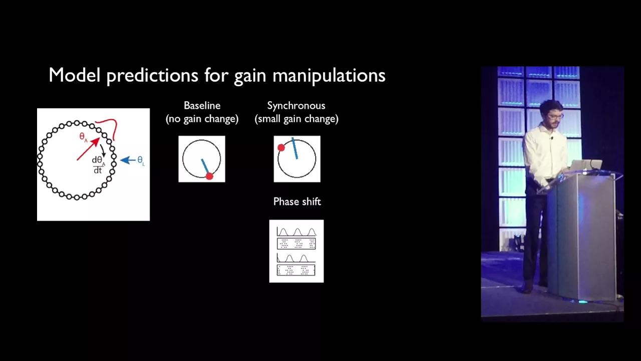
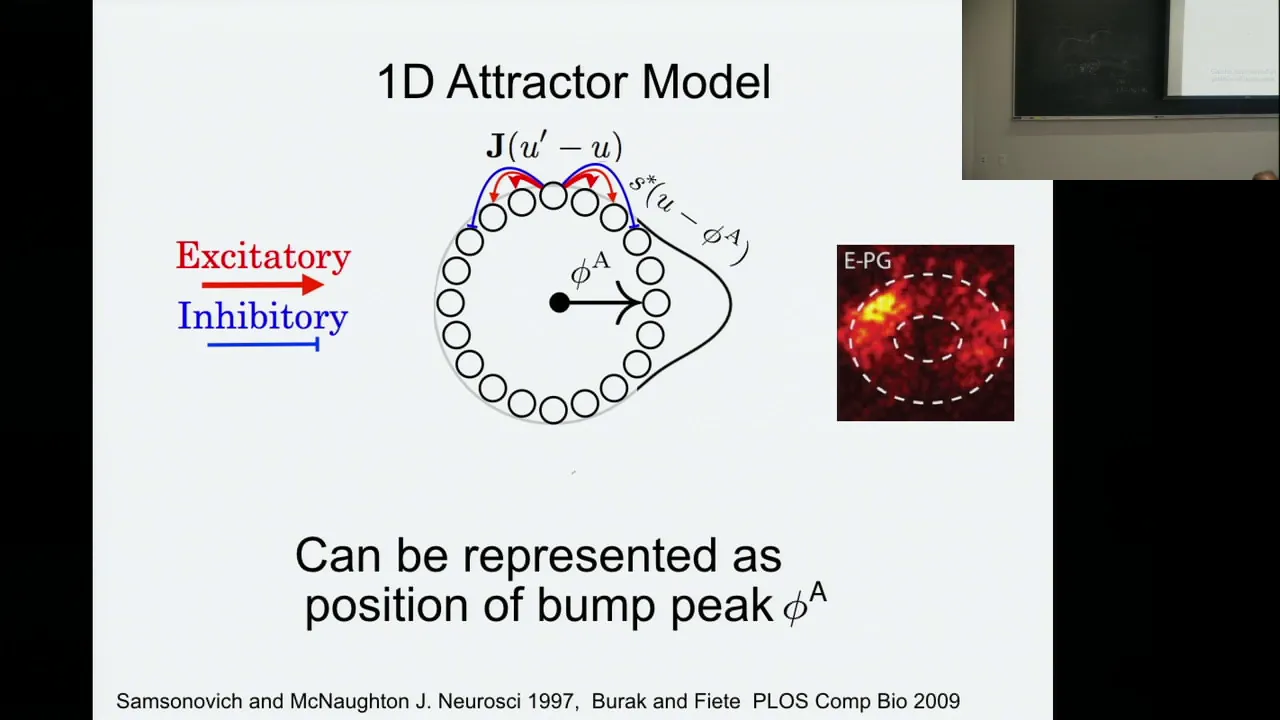
[00:00:00]so I want to thank the people who've worked with me on this before I start and the first half was done in collaboration with Brett Geiger at High Point University and then the second part was done with experimental labs at Johns Hopkins University on this Jim Kinnear I'm Noah Cowan and Kachin Zhang and I also want to thank NIH for funding this work so much to imagine for a second that you have to navigate from one point one place to another and your phone ran out of battery so if you don't have Google Maps and think about the sorts of strategies you might use the first might be kind of self localization so you look around at the landmarks that are around you and try to think about where you are in relation to familiar landmarks the second may not be quite as obvious you're probably not going to be continually looking at these landmarks as you move so maybe more on the subconscious level you know what direction you're moving in you know about how fast you're going and you can update your internal sense of where you are relative to where you started from and this is something we call path integration it's something that rats and mice and other animals that we do these studies with have been shown to be very good at and the basic idea is as a calculus idea that we want to update the internal estimate of position by integrating over self-motion information like the velocity and then of course errors are going to accumulate as you do this path integration and so you need an error correction step as well where you again kind of periodically look up at landmarks to correct for any errors in the path integrator today I'm going to focus my talk on the second step of path integration we go to models of path integration this is kind of a typical general form that you would see here I'd looking at a PDE so I've taken the limit as the number of cells goes to infinity you the state's variable represents the synaptic input for this with preferred spatial variable X that spatial variable could be the heading direction it could be absolute location or place it could be phase if this is a model of say red cell so there are many different things it could represent that would be biologically relevant f of U is the firing rates of each cell and the firing rate is convolve dwith this wait tuning curve W of X this is the weight between cells with distance X between their preferred spatial variables B is a tonic Drive and then H is the South motion input so this could have terms in it with the velocity with possibly the acceleration of the animal but importantly this cannot contain absolute locations so nowhere in this model does the system get information about absolute location or about landmarks these are generally considered to be continuous attractor neural networks so the idea here is that the weight W of X is going to be kind of a center-surround connectivity where these are the outgoing weights from the cell in the middle to the other cells on the sheets and the weights are set such that when this cell is active it wants to recruit its neighbors to also be active and at the same time inhibit cells further away from being active and this results in this localized activity bunk shown here in color over the cellular sheet on this activity bump I'll call capital u it can be located anywhere this X hat could be anything over the cell sheet so I just had is typically the center of mass of the bump and because you should you could shift this activity bump anywhere this is called a continuous attractor because it has a continuum of attractor seats right so for a path integration model it has two components the first is translation invariance of the activity bump and really this is saying that we want the path integration model to lie in the larger class of continuous attractor neural network models so the idea here is that when you have a self-motion input as the animal is moving that the activity bump should be translated across the cellular sheet without any mutations the second component in order to have perfect path integration there should exist a constant gain factor G such that the velocity of the activity bump is equal to G times the velocity of the animal in many models G should be 1 but that's not necessarily true the important thing is that G should be constant in time there's a nice mathematical paper from back in in 2012 that show that in order to have perfect translation invariance imperfect path integration these self-motion inputs should be multiplicative in nature in other words it should have this form where the velocity is multiplied by some function of the states for our system the model would look something like this notice here that G this gain is an independent parameter in the model it does not depend on the other parameters such as your weight tuning curve and to think about how this model works we consider this whole thing to be an effective weight and so instead of just having this weight even weight tuning curve here the system learns this effective weights that is proportional to the gradient of W and scaled by the velocity so that when the animal moves left because of these weights you see a shift of the activity bump to the left and the opposite happens when the animal moves to the right so one more thing on this slide um this model works beautifully mathematically and because of that there are numerous mathematically and analysis studies that use this model to look at things like robustness to noise but there are some issues with it in terms of how biologically realistic it is so how realistic is it for the system to learn the gradients of the weights and for those weights to be scaled on the time course of the animals velocity so because of this many models particularly those that are based on numerical simulations use an additive self-motion input of this form so importantly this H now does not depend on the state you it's not possible to get path integration with an additive model if one just has one group of cells and so what people typically do is to have two groups of cells the weights are shifted no longer do we see the gradient vector but the outgoing weights from Group one are shifted to the right by L from there two are shifted to the left and now these self motion inputs are opposite here so that group one is more tuned to movement to the right route two is tuned to movement to the left and so when the animal is moving to the left the activity bump of group two is slightly larger than that of Group one and that causes the activity bump to move to the left and the opposite happens when the animal needs right and one can extend this idea to two dimensional space by having four groups of cells one for north west south and east so while this model has been shown through simulations to do a very good job of path integration there's not nearly as much of the mathematical foundation for these models as there is for the multiplicative model and so we've set out to provide a rigorous mathematical analysis of this model and what I'll talk to you today is some of our results from from looking at the shape of the moving activity bump any intrinsic errors the system has even when you don't have any sources of noise and in what parameters can minimize those errors and maybe most interestingly how does the gain depend on the model parameters and the multiplicative model the gain is an independent parameter itself but here there's no explicit parameter for the gain it depends in a complex way on on all the model parameters but before I go further we we've changed slightly a definition that's typically used in the literature typically when people talk about a continuous attractor network with two groups what they mean is that both u1 and u2 stay on the attractor but for us we define this translation invariance as the average activity bump remaining on the attractor the idea is that a downstream network of neurons that wants to read out the encoded variable might get inputs from both u1 and u2 and so perhaps the average is more important than each group individually and then we define two errors first is the error in translation invariance we denote this by V and then the second is the error in path integration which is the true gain minus this constant gain factor which we define as the gain if we had perfect translation invariance it's not a given that we could get a constant G not even if V were zero but we will show you a condition for which you do get a constant factor G not okay so this is just a reminder of our dynamical system we begin our analysis with the on sots that UI is capital u plus or minus G Plus V so we have an opposite effect and then as shared effects to analyze the opposite effect we look at the difference in the two states and we find that G is flat spatially and it tracks these self-motion inputs H so to see how this works visually in this simulation we start with you want to new to both at this equilibrium bump capital u and then we applied to it of loss a constant velocity inputs and we see Group 1 gradually increasing to u plus h well group 2 decreases to u minus H here we compare u plus GT 1 and u minus J 2 u 2 and we see right away that this term G is much much larger than this shared term V V is the difference between the solid curve and the dashed curve in both so it's very small relative to the size of the activity bop I'll return in a minute to talk more about V but first let me talk about how we compute the gain I don't have all the mathematical details here but the idea is that we do a Taylor expansion of this considering G and V to be small perturbations and then we use linear operator theory to get this expression for the game we find Rho G over tau V Plus this oh of H squared error term so H is again that self-motion input it should be fairly small relative to the size of the activity bump itself what we found is that this error is 0 when V is 0 so this is an error entirely dependent on the errors and translation invariance we have this new term here this Rho factor which is given by this quotient here the brackets indicate the L to inner products given a constant velocity RG the opposite effect should converge to H which is alpha V and so we find this constant game factor G naught is Rho alpha over tau that's just what this term becomes so before we consider a time varying velocity and put let me just show you on some examples so here I look at three the most commonly used weight tuning curves the black is a cosine the red is Gaussian and then the green is a Mexican hat function the cosine and Gauss are often used for head Direction cells or placed cells the Mexican hat is based on a simplification a 1d simplification of a grid cell network and here are the three equilibrium activity bumps for these three wait tuning curves I set the parameters so that they would all have about the same peak value some example trajectories so this is a smooth velocity but it converges to a constant here when the the H is 0.1 that's about 15% of the peak of the activity bump so so pretty large compared to what what people usually consider and we still see very good agreement between the black which is the actual structure E and the X hats which is the encoded spatial variable when we look at the errors we see they're pretty small about 2% for translation invariance and up to 3% for the game okay so moving on to a time-varying velocity inputs if we go back to this gain equation we see that we have this G of T divided by V of T and in order to have G naught as Rho alpha over tau we need G to be alpha V so going back to this equation and using integration by parts we find that our equation G looks like this where it has this alpha minus beta term here and so we conclude from this that ideal path integration in order to have that constant G not requires a balance of velocity and acceleration inputs or beta equals alpha so this is really an interesting result it's not one that we expected in the multiplicative model the ideal path integration requires no acceleration input whatsoever and in the additive models typically people use only a velocity input so this was a surprising results and I'm going to go through these slides rather quickly but just to show you an example I gave it a sinusoidal velocity input and then compared what happens when beta equals alpha you see exact agreements when there's no acceleration input in blue you see this lag of the encoded spatial variable behind the tree and we can get an exact analytical expression for the phase shift and for the difference relative error in platoon of the response x-hat compared to the true why okay so what is an explicit expression for the gain in other words how does the gain depend on the model parameters we found that we could simplify this under the condition that WD involved with F prime of U is proportional to u prime and looking at this expression you'll see that minus Rho will be that constant of proportionality to determine when this condition holds we did some Fourier analysis and found that the condition holds if and only if this expression holds for all N greater than or equal to 1 and looking back at our three examples that really depends on the decay rate of these coefficients w hats we find that it holds exactly for the cosine because it only has one nonzero Fourier coefficients it holds approximately for the Mexican hats and not at all for the Gaussian so the condition really depends on how broad or narrow the weight tuning curve is hmm for the example of the cosine weights the parameters were interested in are M the scale factor of the weights this shift parameter L and this tonic drive B and when we follow through with this Fourier analysis and simplify we get this explicit expression for the gain there is a term R here which is the radius of the bump but we find that this equation holds well even if we hold our constant that's this dashed red here so we find that the gain is inversely related to the tonic drive V is roughly linear in L and decays linearly and and we have similar expressions for the Mexican hat tuning curves as well okay for the sake of time I'm gonna I'm gonna skip this slide this looks at the spatial properties of that function V and this concludes part 1 of my talk this is part of the results we've had from this rigorous analysis and the gain itself is intrinsic error is o of H squared and we find that this error in V is o of H squared when that condition 1 holds in particular and we've derived an explicit expression for the game the next thing I want to talk about is some numerical simulations I've done with a path integration model of grid cells using that Mexican Hat tuning curve and the predictions I've made for a particular experiment that my collaborators are running so they call this thing that dome and the idea is that as this animals as rat moves around the dome they projects cused up in this virtual reality environment and they control the queues as a function of the animals movements and what they've been able to demonstrate with this experiment is that they can actually recalibrate the gain of the path integrator based on the experience within the dome and so I've been working to develop theories of how this recalibration takes place one big question is where it takes place so one can imagine a recalibration in the upstream head Direction cells or speed cells or there could be a recalibration within this grid cell network itself which is typically considered to be the path integrator so just considering those two alternatives I've made some predictions for how we could differentiate between them so the idea here on the top here we have this the population activity pattern of all the cells in this two-dimensional array and as the animal moves the south motion input drives this capital u in response to the animals movement here in physical space so this is the population lattice and down here is the activity of one single neuron marked by this white asterisk and every time an activity bump moves through the asterisks you see that this cell is active by just fast-forward to the end of this video we see this nice hexagonal lattice in the single neuron response similar to that at the population lattice the gain of the path integrator defines the speed of the lattice translation the speed of the animal can also be given by the period of the population lattice this distance here divided by the period of the single non-response so I'm going start this video and then we'll talk about it so this is the video you just saw in the far left and on the right I'm looking at two different things that could happen within the network due to the game recalibration experiment the first thing that can happen is that the network could change its perceived speed it thinks that the animals going twice as fast as it was originally and so we see these translations have increased by a factor two in terms of their speed on the right the speed of the translations is the same but the lattice itself has compressed this period has changed and so here's what happens at the end of the movie the interesting thing these are two completely different mechanisms for a recalibration one is an increase in proceed speed one is no change in perceived speed but a compression of the lattice and yet the single neuron response looks very similar and this becomes even more complicated because we don't have access to the single neuron response we have access to this under sampling of what we perceived to be the single neuron response this under sampled hexagonal right and so we've developed some algorithms for inferring this full single neuron response grid pattern from this under sampled tract and made some predictions about how we can determine a distinguish between what's going on in the system when we get the data that they are going to be giving me as soon as the lockdowns lifts up so if a recalibration occurs upstream there should be no change in the population lattice and so for the single non-response we should see no change in pairs of collective cells and no change in the relative phase of cell the cell pairs but if there's a change in the spatial profile of the weights that will decrease the grid period and lead to changes in both the pairs of themselves and the relative phase of cell the cell pairs and finally if there's a change in the strength of the leads then that will not lead to a compression in the population level but you'll see a smaller radius of each field and so that might decrease the number of positive pairs while having no change in relative phase of cell to cell pairs and so this is where this this partnership stands right now and making predictions for what we would expect to see as they run this game recalibration experiment and now record from bridge cells in the MSE to try to see kind of these neural mechanisms and the idea is once we get that data in and can test these various predictions and identify where the recalibration is taking place we can go back to these attractor Network models and modify them or adapt them to have some biologically realistic mechanism for the game recalibration so thank you for your time and I'd be happy to take any questions that you have luckily thank you very much Katherine so does anybody have any questions please either raise your hand or indicate in the chat I guess a kick off if everyone's feeling a little bit zoom shy and these three different underlying mechanisms for the recalibration do you have a feel for which one might be the most biologically plausible or would they apply in different circumstances or there's sort of different causes for the recalibration right I can certainly tell you which would be the simplest so that the simplest recalibration would be one one that's upstream although it's kind of just leaving the problem further upstream and then saying well how do those cells recalibrate the difficulty with recalibrating in the grid cell network is that these are attractor networks and so if you have heterogeneity in the weights you could lose the this capital u right you could lose attractor pattern of these exciting companies hexagons and so you know there are things I've been looking into in terms of how to make this is some more robust to heterogeneity this is something that a lot of people have looked at that would permit some sort of a change in weights it seems like something of this form might be easier just to change the strength of the weights as opposed to the spatial profile so so just from a practical standpoint of how I would model this it seems like this change in the spatial profile would be the hardest but then on the flip side when we were initially talking about this with the experimenters we were talking about it a lot in terms of how the grid might compress mm-hmm the the period of the grid is inversely related to the gain and so one idea that people typically think about is that these different modules of grid cells that have different periods have different gain factors and if we're changing the game we should be changing the period of the grids and so that was kind of an initial prediction and so so the difficulties that lie in the modeling side and then trying to think of biologically realistic implementations don't necessarily mean that we shouldn't think about it and look for it yeah ok great ok are there any other questions thank you very much for a very nice talk umm so do you have a feeling from from the analysis about robustness about how robust each of these different mechanisms are and to noise or just in terms of the general overall yeah so I didn't sure that here I have done some robustness studies in particular for the Mexican hat weight tuning curve because that is kind of the simplification of the grid cell model that I'm particularly interested in so it is fairly robust to changes in an El this shift parameter and and in the strength of the weights there are critical values where you you see this kind of bifurcation and do lose the attractor network or you see this dramatic change in the period when you change these parameters and so I've been able to identify pretty well kind of the range in which you can change the parameters and it certainly gives you plenty of room to have some significant changes in the game maybe not a significant by themselves and in what they're seeing in in the experiments but we need the data to know that but there there is also a complication when it comes to looking at robustness for it for grid cells so this kind of gets into the into the weeds a bit but whenever you have this attractor Network you can't have any sort of heterogeneities at the boundaries because it will cause deformities throughout the entire cellular sheets and so the easiest way to get around that is to have periodic boundary conditions but if you'd have periodic boundary conditions you're enforcing a particular rotation to have lower energy than other rotations and so it forces the B grid to to not rotates whereas if you do other methods like using some sort of an envelope function to kind of taper away the effects at the boundary it's very prone to rotation and so in general it would be unstable in terms of a rotation of the of the grid and and that complicates things since we are looking at kind of this circular track and you might have a recalibration of head Direction cells a rotation might occur as part of the recalibration and so that makes it complicated in terms of being able to read out predictions from the model in terms of what you'd expect to see in the system due to just lack of our bus'ness versus due to something real happening in the gain recalibration thank you very much