




![[4] Tout Savoir sur les Pixels, l'Échelle Hounsfield et le Fenêtrage en Tomodensitométrie !](https://i.ytimg.com/vi/veO_clVHxN0/maxresdefault.jpg)





![Parellel Beam CT, Fan Beam CT and Cone Beam CT geometries [Radiologic Technologists / Radiographers]](https://i.ytimg.com/vi_webp/KhOCZsl28dg/maxresdefault.webp)

![Tomographic Image Reconstruction: Iterative Methods (Part 3) [L30]](https://i.ytimg.com/vi_webp/aES-vIndNyY/maxresdefault.webp)




![[19/05/2021] Severo Ochoa Seminar by C. Lee; "Shape prior metal artifact reduction algorithm..."](https://i.ytimg.com/vi/OhKPSg2r7ws/maxresdefault.jpg)




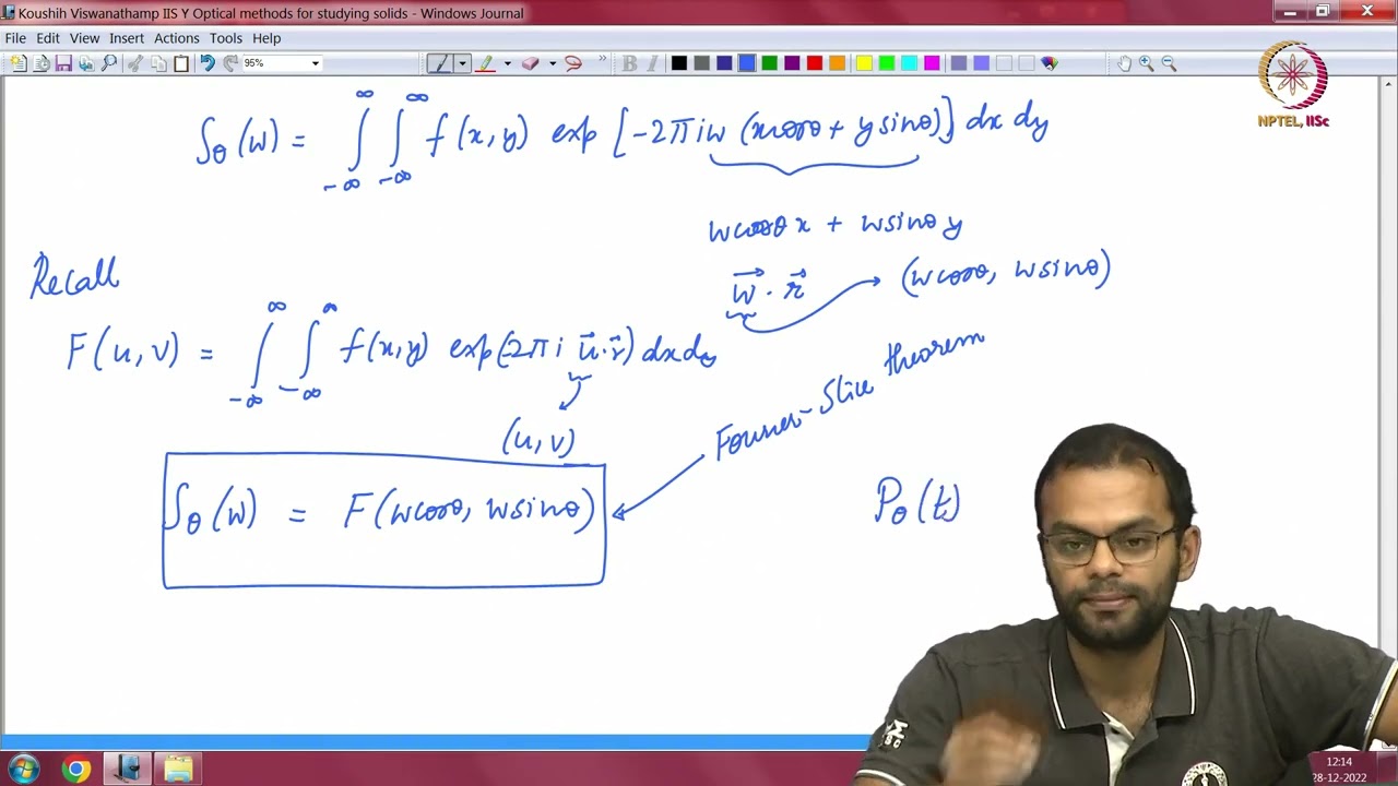
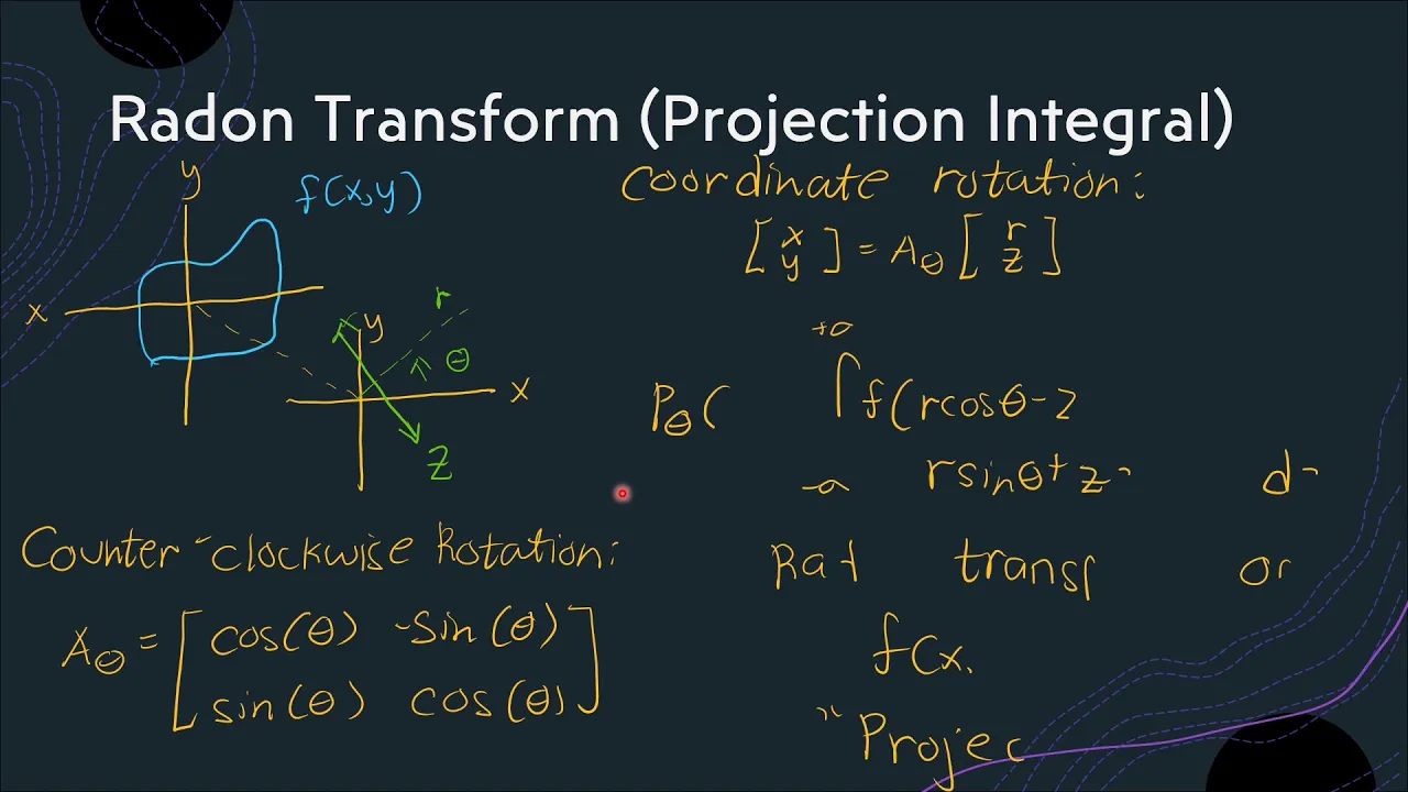
This lecture explains how CT scanners reconstruct cross-sectional images of the body from X-ray projections using the Radon transform and filtered backprojection algorithm. The Radon transform mathematically represents projections as line integrals of the image intensity along lines parameterized by angle θ and perpendicular distance ρ. The Fourier-Slice theorem establishes that the 1D Fourier transform of a projection equals a slice through the 2D Fourier transform of the original image. Unfiltered backprojection causes blurring because it oversamples low frequencies at the center of the Fourier domain; filtered backprojection solves this by multiplying each projection's Fourier transform by a ramp filter (|ω|) before inverse transforming and summing over all angles, producing a sharp reconstruction.
Image Reconstruction from Projections: Radon Transform & CT
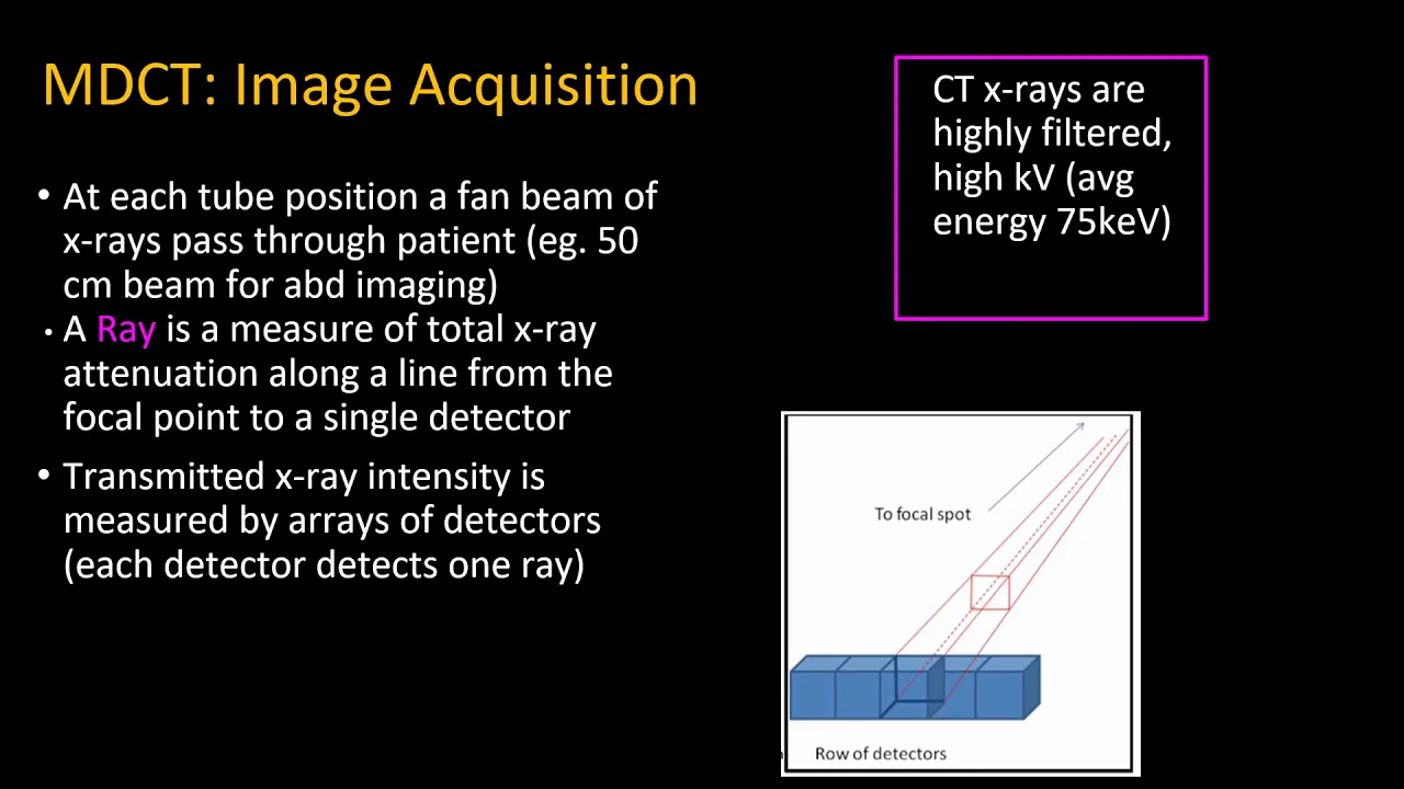
Added:okay so this lecture and the next are uh kind of a offshoot of image processing which I would call Image Reconstruction from projections and basically this is the foundation for how cat computed axial tomography or CT scanners work okay and so the idea is that you know I think I drew this kind of initially you're the patient you're lying on a kind of a table there's like a little bed that you're lying on this is a pretty crappy picture and the idea is that you go through this machine I'll show you a couple pictures of real machines in just a second that is scanning kind of cross-sections of your body okay with projections of X-rays and then using those projections it reconstructs the interior of of your body okay and so um let me show you a couple examples what we're going to talk about first is so here here's Yeah couple pictures from the book okay so there are lots of different geometries for how this uh process of x-rays going through the patient can occur okay and so what we're going to talk about today is the upper leftand case where basically you've got a set of uh like you've got an x-ray source that is pushing parallel beams of x-rays through the patient and receiving those at a detector okay and then next time on Thursday we're going to talk more about these kinds of things where instead of there being a set of parallel beams you instead you have what's called a fan beam a set of beams that is kind of pushing out from a central source and directing diverging Rays out towards the patient okay so there there are several Generations they call them of CT scanners and so you'd kind of call this up here like generation one and this is like generation 2 Generation 3 Generation 4 and probably most of the stuff that you'd see in a you know hospital or clinic today is along the lines of this scanner here uh although if you go to a really good Hospital like you know Mass General Hospital or Memorial St count Cancer Center they're going to have even more advanced uh stuff and that's kind of what we're going to talk about next time okay so here's just a couple pictures um so here's what the inside of a cat scan machine looks like and so what you can see here is this is a x-ray source and this is the patient bed and the X-ray source is going to shoot beams through the patient and over here behind these fans is the set of X-ray detectors and this whole thing spins around the patient very fast and so here's a a video of the actual uh spinning cat skin and so you can see that once it gets up to speed it's going pretty fast right so uh you know think about that the next time you're inside the scanner that this thing is this huge chunk of metal that is spinning like crazy paent goes here there so um yeah all right I don't think we have to watch the whole minute of this so okay all right so that's the good news the bad news is for you guys that this is a very mathematical uh lecture this one and the next one are going to be the most intense math that we do for the whole course Okay so get ready for derivations and integrals and all that good stuff okay but by the end of it at least you'll know like how this stuff actually works okay so the principles of um how this works have been known for a long time so basically um there's something that we're going to talk about today called the radon transform and that's been known since like you know almost 100 years okay but of course they didn't have the ability to create X-rays and deliver them and push them through patience until much later and so um you know basically the 19 the 1979 Nobel Prize was given to two guys Cormac and houndsfield who were the ones who decided or who who were able to make this uh extra Imaging process practical in real medical medical applications okay okay so let's just consider one cross-section of the patient unfortunately you can still hear I'm kind of froggy so sorry for my voice okay so here's the patient and let's suppose that the x-rays are coming at the patient in this direction okay and so the whole premise of this is that if the X-ray doesn't hit the patient at all it's just passing through the air and its energy is not attenuated at all okay whereas as the X-ray is passed through tissue and flesh and Bone some of the energy the X-ray is absorbed by the patient okay and that means that if I think about an absorption profile that basically nothing is absorbed out here and then as I kind of go through the center of the patient I have you know more x-rays being absorbed okay and so let's think about this in the sense of um M lab right so all we're doing basically is we're taking the you can think about taking these image intensities along each of these lines and adding them up or integrating them to produce kind of a profile and then by going along different directions of the patient we got different profiles and so the premise is if we see enough of these profiles kind of intuitively we should be able to understand how to reconstruct inside the patient okay and so here's a simple case you know let's suppose that the patient looks like a circle right white circle on a black background so if I project x-rays this way and integrate I'm going to get something that kind of looks like uh you know this integral right and if I project x-rays this way I'm going to get something that kind of looks like this integral and one idea is what if I were to take the things that I see and do what's called back projection okay so the idea is that I could look at the um kind of pushing this profile in the same direction of the x-rays to produce kind of a smear and this is called back projection we're going to talk about this a lot more so don't get worried right now but the idea is that what I could do is I could say okay I could kind of produce a smear that kind of has the same cross-section going this way and I could produce this kind of smear I guess I can draw it like this that would have the same kind of cross-section going that way and then I could say okay now I look for the places where these two things intersect right so if I add this plus this then I get something that looks like big in the middle and fainter in the other areas right so kind of what I would C would be something that would look kind of like a you know a radially symmetric bump I'm going to show you a real example so that you don't like just try and figure it out from this basically this would be you know the most overlap between these things and I have a little bit less overlap here here here and here so let me just show you a mat lab example of this to make this more concrete because I know this is bad when I'm trying to draw it on paper Okay so here is a exact replica of what I just showed you right so here's my simple image okay and what I can do is I can plot the integral of that image in whatever Direction I want okay as we're going to talk about in just a second that's related to What's called the radon transform so um mat lab has a function radon that helps us with this and so what I'm going what I'm going to do is I'm going to say um Let me show me what the uh plot looks like if I were to integrate this picture straight down well it looks like the integral of the circle right and so um you know it's nothing in the black areas and then it ramps up until I've got the full radius of the circle and then it ramps back down right and if I were to plot that at any angle I get the same thing right because no matter what degree I project that Circle from I'm always going to get the same you know the same basic projection right and so if I were to have a different image so let's look at this guy so here's a slightly different image where I've got a big circle that's white and a smaller Circle that's kind of gray right and so here if I were to project this image uh let me first do it like this right if I just project it straight down I would get two little Peaks right one corresponds to the big white circle that has a lot of intensity one corresponds to the little gray Circle which is smaller and is also darker right so if I project it straight down let me just remind you what the um original image looked like right so if I were to project this image straight down I've got big white circle and then little gray Circle if I were to project it left to right the other way then I'm going to get something much different right so if I project it the other way what I'm going to get is here let me uh put that image back up again so here if I project it left to right what I'm going to get is that the little gray circle is going to overlap the big white circle and I'm going to get kind of this extra little Peak that comes in the middle so instead of looking like a straight you know quadratic curve instead I've got this little hump in the middle okay so in this in this view I can't really disambiguate the small circle from the big circle right they're not very well separated so the idea is okay well what if I were to take the projections let's let's go back to our first Circle okay so so what if I were take my projections for all the different angles and smear them out in the appropriate directions and add them up okay so here's an example of that so what if I were to take for example [Music] the and don't worry about these um functions right now so what I'm going to do first is I'm going to take uh my original image I'm going to project it at 0 degrees and then I'm going to look at that as if I were to smear it out smearing it out makes a kind of a vertical up and down white bar that's like saying take all that Circle energy and spear it around okay and let me just make sure that I've done this like this right it actually looks more like this because there's more energy in the middle and it drops off to the sides right now if I took the smear from up and down and added it to the smear left to right what would I start to see so what I can do is I can say okay I'm going to take a selection of uh thetas angles that is and I'm going to uh take my rayon transform which I'm going to explain more about so don't worry if if you don't understand what that means quite yet and then I'm going to add those two things back up so here is the sum of the two smears right so so this gives me something that is kind of close right because I it already tells me there's a blob in the middle of the image right but the fact is that this guy you know has these these cross arms that come from places where there's only one active smear right so maybe I could better if I were to make my Theta sampling a little bit finer right so let's suppose I took a couple more angles and add them together from different directions well now I'm starting to get something that again the the arms are kind of fading away a little bit and if I keep on doing this to say okay let's suppose that I sample this every 20° or so then slowly and surely uh circle is starting to form right and if I take this to kind of the the limit and I say okay now I'm just going to take every degree for example a really fine sampling of theta and I show my sum well now actually this looks kind of like what I started with right but there's a problem right the problem is that there is this kind of Halo right and also I know that I started with a circle that was uniform intensity right but this circle seems like it's a little bit brighter in the middle and a little bit darker at the edges right so there are a couple troubling things the most troubling one is this fuzzy Halo because it turns out that theoretically no matter how many how fin I take my Theta sampling I'm always going to get this little blurry halo around the object okay and we're going to explain the reason for that a little bit later in the lecture um because you can imagine that again we're using this for mostly medical treatment and diagnosis right so you don't want to have something where the doctor overestimates the size of the tumor or doesn't see where it is because it's too blurry right I could do the same thing with the um I can do the same thing with the other image so let's suppose I take um that two Circle image again here's another case where if I don't take enough projections then my kind of blurry and smear part is almost threatening to overcome this this guy here right and so I don't want to be in the situation where I miss something because the artifacts in the Reconstruction have have overcome something that is maybe a a subtle light thing that I want or a dark thing that I want to find and here's another example if I take all the projections I can do a little better but still that you know Moon orbiting the Earth there is definitely a lot darker than it was the original image and it's almost subsumed by the same blur that's going around the image okay so this is the issue how can we do better than this okay and so the answer lies in the formulation of this problem as basically a mathematical construct okay so here's the math of how it works okay so this is kind of related to the Huff transform that we talked about a few lectures ago for detecting the lines right because again here we're talking about line is going through an image and so this idea of parameterizing a line is important so if you recall for the Huff Transformer we were saying okay suppose I've got this line here okay and this may be slightly different than how I did it for the Huff transform but either I could talk about this line as a slope and an intercept right we kind of talked about how in image processing sometimes it's easier if I talk about this angle Theta and this perpendicular distance row right the Huff Transformer is basically a way of taking a line and mapping it into this row Theta space okay and so in row Theta terms the line is described by this formula x cosine theta plus y sin theta equals R these are two equivalent ways of representing this line okay and so if I tell you a fixed X I'm sorry a fixed Theta and a fixed row that corresponds to some line going through the image plane okay and so let me just draw another more complicated diagram right so here what I'm going to do is say let's suppose that this is the XY plane here I'm going to use again cartisian coordinates here is the patient kind of a squiggly patient and so let's suppose that I've got some uh what the best way is here suppose this is the Direction I'm going to project okay so I'm going to push x-rays through the patient and image them onto this plane okay so if I think about it right if I go back to my my picture here I have to figure out what are the rows and the thetas corresponding each of these lines right so the has to do with the angle of the perpendicular so if I think about this line here this angle is Theta okay and then each of these guys is a different row right this is like Row one row two Row three row four all with the same Theta so I can say okay this is like the the C projection that I'm taking of the patient and I'm going to call this function this projection function G of row J Theta K right so J is indexing this guy and K is indexing this guy and so for a fixed row comma Theta that's like specifying one particular line and that gives me this value here which is like you know G of Row 3 comma Theta K okay so comments or questions about the setup and just to make it a little bit nicer here is a you know picture from the book that is exactly what I tried to draw in my Clumsy way right same thing okay so what next well first of all let me see if I can describe how do I get this number okay it's like an integral it's an integral along a line going through the patient so this is actually something that you may remember or may not remember from like calculus 2 perhaps or calculus 3 a line integral okay and so let's write down what that actually means so what I'm going to do is I'm going to think about this I'm going to say that my G of row Theta is like an integral across the XY planes I'm going to have a dxdy here and I'm taking the image and I'm integrating that image only where I'm along the line and so I'm going to kind of use this kind of abusive notation here to say here is that line I'm just going to add a Delta function here so it's basically saying where this inner condition is true the Delta function is firing otherwise it's not right and this is called the radon transform and that's exactly what I was doing with mat lab right I was calling this function called radon that was doing this integral for me and of course you know in the discret world all of these integrals are replaced by double sums but we're going to keep everything in integral world this lecture in the next because it's much easier to talk about with continuous time okay so questions or comments yeah soy that's the intensity of that pixel yes this is this is basically just like our usual original image right then the Delta function is just on the line so again if I think about this line here is described by this equation right and so what I want just to say I only want to look at the X and Y where this is true right so I'm kind of moving the row over to the other side okay other comments or questions okay so we can think about just like for the Huff transform right this is not the same as the Huff transform but just like for the Huff transform you can visualize this function of row and Theta as an image right and so if we do that that's what's called the the sinogram of an image and actually the word comes from the soo part comes from uh not signs and cosiness but sinus like the sinuses in your head right which is a hole right so this like a way of visualizing the holes in the image apparently is where the sinogram came from and so you can do this with the raden transform I wrote a little function to make it easier myself so all I'm doing if you see what I'm doing here is this is just like basically cutting paste from the mat lab help I'm just taking the rate on transform and I'm IM showing it and putting a color bar on it so not anything fancy and so let's take a look at the cogram of my original image the one with the circle well I guess uh looks like this right so if I do another figure so again way to read this and I guess that I kind of uh maybe shouldn't put this quite side by side because I made it so you can't see the labels so here the x axis let me see if I can kind of make this a little bit better you know I'm just going to this again because I so the x-axis is the Theta which is degrees and the Y AIS is basically the row which they're here calling X Prime and so again we know for this circle that no matter what Theta I take I always see the same projection right so if I was to think about taking a cross-section of basically a vertical line through this I would get one of the pictures I showed before that looked like the the hump that is the same from any angle right on the other hand if I were to take my other image this guy and look at the sinogram of this this would be very different so that looks like this so again the way I think about this is that from pushing the image just down onto the x-axis I would see the big circle followed by the little circle right in the middle if I were to push it across 90° what I would see would be the big circle and the little circle overlapping which was that little extra hump that you saw and then as I changed the angle you know basically there's there are some points of view where the little circle doesn't overlap with the big circle and there are some where it does right so kind of what you see is this kind of Two Moons you know overlapping with and of course for a real image the sinogram looks even more complicated but if you know what you're looking at you can kind of think about interpreting why the image looks like this right and so one of the homework problems is basically to take another image and look at the Sy sinogram of it I believe and think about why does it look like the way it looks right okay so questions are comments about this picture okay so my first idea was to see what would happen if I were to take these projections from different angles smear them back project them and add them up right so mathematically what would be happening there so so say we have a set of projections right I'm going to assume here that this is like a continuous function of row but a discrete function of theta for a set of angles Theta K between Z and Pi the reason only going halfway around the circle is that I get the basically the same projection if I project from up to down versus if I project from down to up right so I really only have half circle of unique projections and so now what I want to do is I want to take my you know here's my G of row comma Theta K and I want to kind of smear it which means that for each for a fixed row what I want to do is I want to basically kind of like copy this pixel along this angle right so I kind of want to smear this value here along this direction to create a new image and so for a fixed value I'm going to fix one of my rows and one of my thetas just copy this value into the image along the corresponding yine okay and so again the corresponding line is x cosine Theta + y sin Theta = row and so basically if I fix these things this tells me which x's and Y should get that bit of intensity and so one way of saying this is that the smeared image which I'm going to call uh so this is basically the back projected image at Theta is equal to taking this profile and smearing it in this way right so this is like saying okay what's happening at XY well I have to figure out for this XY what is the corresponding Row in Theta right this is the corresponding row and I already know the Theta because I'm telling you what Theta comes from right so here I have to know which of the projections lines up with each of the thetas right and so then if I want to reconstruct um basically the sum of back projections which is going to be basically uh just this I take all my thetas that I got and I add these images up and those are the kinds of pictures that I was showing you before those are actually called linrs okay so this was our first attempt right and as we saw visually this has this problem with blur okay but at least this is what's mathematically going on so let me pause and ask any questions about this yeah so the idea is that this is kind of one single smeared projection and then what I was showing you earlier was if we add these projections up I start to get that blurry image right okay but the incs are a specific right so I have a set of specific Theta so I have basically a discret set of theta that I'm adding up from different directions right I I could make this an integral if I had a continuous set of theta but I'm assuming that I'm just choosing some set of other questions okay so now the real fun begins so uh we have to understand how can we do a better reconstruction and so in order to understand what was going on in the first place we need to go to The fouryear Domain everyone's favorite place and we're going to prove something called The fouryear Slice theorem okay so the fouryear slice theorem is pretty cool sometimes it's called the uh projection slice theorem and it's going to give us the relationship between the for your transform of each of these projections and the original image that we were trying to reconstruct in the first place okay so basically it's a relationship between I go back to my picture here the idea is that this image has a 2d for your transform right each of these projections has a 1D for a transform and there's some notion that those two things should be related somehow right I should be able to get this for a transform from this 2D for transform okay that's the idea okay so let's uh consider a fixed angle theta's uh projection oh no seems like my pen is running up this is the worst time and take the both of my pens are running out uh oh let's see what we got in the tray here nothing good pencil really see how this comes up the 1D for your transform I guess it's very nothing oh it's all right with respect to to row okay so basically this is going to be like the thing that we use to take our for transform and so um this is kind of like row is kind of like the time domain and I'm going to convert that to what I'm going to call Omega which is going to be kind of like the interpretation of the frequency domain Okay so so I'm going from my G row of theta to Capital G Omega Theta Theta is just coming along for the ride to remind me that I'm fixing that particular angle okay so my G here is just our usual for a transform this guy eus J 2 pi Omega Row D okay so this is nothing new if anyone has a thicker pen I will take it okay so now what I'm going to do is I'm going to substitute in what do I know about this for your transform okay well I'm going to write what I know about the rad on transform well let's go back here I Define the radon transform over here right so I'm just going to plug this in to this to make it even worse integral so let's see that's like saying that I have an integral out here which is going to be my D I have the integral for the radon transform this is my original image here is this Delta function here is my dxdy and then I have eus J 2i Omega Row D R then I have to apply my usual trick which is to switch the rows and the x's and y's right so I'm going to again I have a triple integral where I'm going to take out the XY part so let's see I can take out this part this doesn't have anything to do with row then I have to have this thing then I have dxdy okay and now I know what happens when I have the Delta function right so all I do is I say well this integral purely uh exists when this guy is zero right so I plug in the row for which this condition is true so I get this thing e the minus 2 2 pi J Omega when is this going to fire it's going to fire for these particular values of X and Y DX Dy okay next now I can do a little change of coordinates okay so instead of using uh X and Y I'm going to use polar coordinates so I'm going to say basically um actually I'm going to change the actually I'm not going to really do this at all I will do that later I'm going to write this in a slight different way I'm going to write it like this eus 2 pi J and then I'm going to write uh write it like this ux + VY DxD so for this to work my U has to be equal to Omega cosine Thea and my V has to be equal to Omega sin thet okay why did I do this because now this thing looks basically like uh a forer transform a 2d for year transform so what I'm saying is that this actually is exactly the for transform of of the original limit right this is like the for your transform of the original image along the line uh U equal Omega cos Theta V = Omega sin Theta so this is pretty exciting what this means is that here's my projection part right so here's this guy I take this is my projection and what we're talking about is what do I get when I take the for your Transformer of this onedimensional signal what I learned was that's like taking you know let's call the for transform this um just like a little for transform like this I guess I should have so just called f of UV and what are the UVS I'm evaluating I'm evaluating at this exact line here so if this is my you know weird complex value for your transform that's like saying that the 1D for your transform of the projection equals the slice through the 2D for a transform of the image at basically the same angle right so this this makes it very immediate say okay if I want to get the 4 transfer of this I take the 2D 4 transfer of the image and I just look at the corresponding diagonal line going through the center okay so in principle every time we take a projection we're getting another slice through the for transform and this is kind of is the intuition for why I should be able to reconstruct from projections because if I sample finely enough I'm going to get all the slices through the for transform that I need okay so that's good right that that's the intuition for why this should work and why I need to have a lot of thetas to make it work right and this picture also tells me why I have the blurriness problem why I have this incorrect reconstruction the reason is that in practice what I have again if I look at this is the uh if this is my 2D 4A transform of the image what I'm getting is you know I'm getting kind of a slice of the transformation here and I'm going to to slice the transformation here I'm going to to slice the transformation here and so on and if I add all these slices up directly the problem is that the middle of this sky is kind of like over represented right because all the slices overlap at the middle so that means that there's too much stuff being added up in the middle right maybe around the edges I've got the right thing but in the middle each of these guys is adding up more than it should right I really only want to have the middle sampled once so this is arguing for the fact that what I want to do is I want to take each of these slices and I want to weight each of the slices so that's it's lower in the middle and higher at the ends right so when I add them up I get exactly the contribution that I want in the middle and everything is even right so uh the idea is that the middle of the 4 transform the 2D 4D transform is oversampled that means that summing up um back projections directly is inaccurate and it's inaccurate in in the way that we saw which is that things are blurry right it's like I'm adding lowf frequency stuff to the image that shouldn't be there right I'm not adding noise like salt and pepper noise I'm adding blur which I know is low frequency right that's why and so the intuition is we should down weight the middle okay and so this leads to an algorithm that is what we do use called filtered back projection right meaning that I'm not just going to add the back projections up directly I'm going to do something to them before they add them up all right so let me pause and ask any questions I can keep my voice going for another 20 minutes I should have brought my huge Gatorade okay so here we go so this is the idea behind what's called filtered back projection so what do we want we want to take my image I guess I should say I called it I right so I want to get back my original image which is just the inverse 4 transform like this right this is our definition of the 2D inverse for transform D DV okay and now I am going to do a change of coordinates right because here because of the nature of the way I'm taking the slices I want to change just to kind of like polar coordinates of the for transform right so now I'm going to do a change of coordinates of the 40 transform to Polar that means that just like what I said before I've Got U is Omega cosine Theta V is Omega sin Theta that means the DU DV is Omega D Omega D Theta right this is just like RDR D Theta from you know polar coordinates right except I'm calling Omega R okay so that means that if I rewrite this thing in polar coordinates I get this so Theta goes from 0 2 pi radius goes or Omega goes from basically minus to Infinity then I have my f then I have my I guess I have to actually can't use UV anymore because I just redefined it U becomes Omega cine Theta Omega sin Theta then I have e to the J 2 pi now I've got kind of a mess up here this becomes x cosine Theta + y sin thet * Omega then I have omega D Omega D Theta right this is like the RDR D Theta okay but wait this is good why is it good it's good because I just came up with this thing right over here right after all this what I came up with was that if I can find my piece of paper I guess I came up with this right this is like saying that this is like the for transform of this guy here right this is kind of I'm evaluating the for transform of the image at this point and the four your slice theorem tells me that I'm asking exactly about this line I know the for transform here it's the for Transformer of my projection right which I called this so that means that by the foure slice theorem for your slice theorem that's exactly equal to the for transform of the corresponding projection at Theta then I've got this junk up here okay and I can make a little bit of a substitution here so instead of going all the way around the circle I really only know that I have to go halfway around the circle and it turns out that projecting this direction and the other direction are basically the same thing so this is a homework problem or possibly an exam problem to show this is true why is this true it's true since if I project from theta plus pi I basically get the reverse projection here it's kind of saying that you know if I have this guy here I get this if I projected the other way I would get this right so it's like I flip the Omega around this way okay so I'm going to wrap it all up what I'm going to do is I'm going to say that this is like equal to the middle guy is equal to this integral where I evaluate along this line right all I'm doing is I'm kind of getting rid of this by calling it row and saying that I've got this integral that I evaluate here and so again if I didn't have this this would just like be the inverse foror transform of each of the projections but here I'm multiplying it by this number right this is kind of telling me that this is how I have to modify each of the projections before I add them up right so here this this is kind of like think of this as the sum you know of adding up a bunch of discrete projections instead of a sum I've turned into an integral so this is the idea is that this on the inside is just the uh inverse for your transform of this guy but multiplied by a filter function absolute value of Omega and so these are what we call um the filtered back projections taking the place of the actual you know originally we were just adding up these back projections instead what I'm doing is I'm adding up these filter back projections so what we came up with is this is the mathematically correct thing to do right because if I go back and look at what started this whole chain was that the beginning of this was the original image right so this tells me how to get the original image from B these are the for transforms of the original um slices okay so I'm going to show you just an example of that in just a second but let me just kind of reiterate the the main idea so overall first thing I do is that I compute the 1D for transform of each projection then I multiply each for a transform which I could call for example G of Omega by this absolute of Omega absolute value of Omega then I take the the 1D inverse for a transform and then I integrate or I sum up over all angles to get my original image and so clearly you know this kind of assumes that I have an infinite number of projections right and in practice I need to have enough projections that I get close to the ideal result okay and for those of you that are still following along heroically one minor comment to make which is if you're really like super knowledgeable about the for transform is what does this you know what does this function absolute value of Omega look like right looks like this and you notice that we never took for Transformers of functions like this back in Signal systems and the reason was that it integrates to Infinity right and that's the kind of thing that I can't take to for transform that's like one of the rules of for Transformers and so typically what happens in practice is that we uh multiply this by some sort of a function that like a window so that what I'm actually multiplying it by is something that looks kind of more like you know like this right this is like what happens I multiply these things together so this could be like a Hamming window it's called the Hamming window and this is to prevent possible you know fore transform kind of uh numerical issues I mean I could just kind of make a box and cut it off at higher frequencies but if I did that I would probably get these kinds of ringing artifacts that we know come from boxes in the frequency domain corresponding to syns and time okay so let's look at some results so luckily you don't have to code any of this yourself right so if I just look at the radon and inverse radar transforms so you can see here that the help for Radon gives me these options right so here what I was doing before was no filter right that's just like adding up the projections directly which we know is bad the default for this function is this Ram lack which is basically just the absolute value of of you know Omega right which is just what I told you about and they say it's cropped meaning I think they just cut it off with a box filter but then you could multiply that by any of these windows to make it smoother so the inverse Ram transform gives you all those options if you like and so let's see what we get so again let's take our uh original Circle and let's take the uh I'm just going to kind of put all this together so let me make a vector of theta that is okay like this and then I want to look at is the uh inverse radon transform of the forward radon transform of the image at these thetas I Supply the same thetas back to the invers transform and I look at this as a image if this worked I should get this okay so then basically this is saying if I only have like 20 projections then I start to get the circle right but this is not enough I need to have more projections so if I were to use uh let's say you know 10° instead things start to get a little better and if I start to use say one degree you know looks pretty good right you can see that there are some you know kind of noisy artifacts here but certainly the interior of the circle looks flat like it should it doesn't look kind of you know brighter in the middle like I did before the edge of the circle is very sharp which is good uh and then you know kind of get these little spirograph looking artifacts that come from you know the diffusion of this hard Edge in the image but you know this is actually quite good and the same thing is going to be true for my other image so if I do uh this guy and then I look at the corresponding High number of theta invers transform like at this right again no problems with pluring no problems with that dark circle getting too dark um but these kind of characteristic diffusion artifacts that come from these hard edges and so um mat lab will also let you you know there's a built-in Fantom so if you just say Phantom of some size what you get is something that is uh kind of like a standard for approximating kind of a I'm not sure whe this is meant to approximate human body but it's kind of like a you know you could imagine that maybe the dark C maybe these are like your your weirdly shaped lungs this is your heart this is your spinal cord the outer rim is your body I mean it's not really super accurate I mean actually this doesn't make any sense in some sense because this is saying that you got a white area like a hard bony shell around your abdomen right so that doesn't definitely occur for humans but you can still show uh you know the Reconstruction of it right so here's the before and after and I guess that the reason that they like this Phantom is that if you look at the uh calling sequence you can kind of tune the contrast of each of these blobs with respect to the background right so you could say okay well how would this perform if these blobs were slightly lighter at some point it would be tough to reconstruct these from the kind of noise that gets added to the image right but you know this is the basic idea okay so comments or questions about this so kind of what I'm going to ask you to do on homework is to basically take a different image take the r transform take the imers transform inter what you see for different you know spacings of theta that kind of thing okay final thing I want to say is just a couple of little uh further implementation notes so so um you know mat lab I believe I could be wrong it used to does this all with ffts right everything is in the forer domain but most CAT scans most CT systems do everything in the spatial domain with convolutions so let me just take what I end up with right this was my final result I had these were my integral of the filter back projections this is where I basically ended up last time except I put a uh I put the window in here too to remind myself that in the real world we have to probably put a window on there so here right what I've got here is the forar transform of something times another function right and so I could say that instead of doing that for transform I could just think about this as a you know this s of row is equal to the inverse for a transform of this guy here and since I'm multiplying the frequency domain this would be like convolving in the time domain or the spatial Dom so I did was basically I removed this complex for transform here and I replaced it with something where I'm just taking every literal projection that I get and convolving it with this other function and then adding those up right so this is just like a kind of a spatial domain version of this um and if I want to be really explicit about it which is even worse it would look something like this so I take this convolved with this right this would be like a 1D spatial convolution so in some sense one advantage of this idea is that if I'm just kind of storing up the sum of back projections I don't actually have to store them all right all I have to do is kind of loop through every projection and every time I get one I do this convolution and I add it to my result right so you know magical notes for when you implement your own CT scanner so no need to uh store all back projections just add them up as they come in um another comment if you were really paying attention is that since this function here the ideal function is zero at this point we really don't know what the DC value of the for transform is going to be so we lose something so since this equals zero at equal Z we lose the DC value in the filter back projection algorithm and all you really do is you just scale your result where you guess what the DC value is right so I think that what you were seeing in those B lab examples was just the result that you got scaled so that the darkest thing was black and the brightest thing was white and it looked fine right but I mean if you were really concerned about not just the structure but also the precise value of the gray scale one of those things that would be a problem and so finally so today's systems use a fan beam or more complicated and we're going to talk about that next time right but the difference is basically that today the future systems instead of just shooting parallel rays across the patient like in this upper left hand quarter instead it's more like the lower leftand corner which is that the Rays from the X-ray Source are diverging that means that we have a different projection geometry and so we can prove I need to decide exactly how tedious I'm going to be in the next lecture about proving what happens with this geometry that a similar reconstruction theorem can be derived and also another way of thinking about is that you can convert this fan beam geometry with a clever resorting of rays into a parallel beam geometry which then you could apply the stuff from today so we'll talk about that on Thursday again that's going to be also mathematically tedious um but on the other hand I have to get to the airport in the early afternoon so I may have a shorter lecture where I give you the high points of fan beam Rec construction and then take off early so we'll see how that goes on Thursday but that's the basic idea so any comments or questions about parallel beam reconstruction really the only thing I need you to know for the exam for example and your general edification is this radon transform so the Ron transform and this notion of reconstruction from Filter back projections that's fair game to talk about on the exam and to talk about in general knowledge the on Thursday is a little bit more out there and you're not going to need to worry about that too much okay so
Up Next
CT Reconstruction: Radon Transform, Fourier Slice Theorem, & Convolution Backprojection
@jpacademia4716
27.4K views•2020-10-30

Elliptic Curve Cryptography Explained: ECC, ECDSA, ECDH
@PracticalNetworking
28.5K views•2024-10-21

Fourier Series Introduction: The Big Idea Explained
@DrTrefor
387K views•2021-05-03

The Mathematical Impossibility of Accurate World Maps
@Vox
23.3M views•2016-12-02
Related Study Plans & Knowledge Roadmaps
Structured learning paths in Mathematics