RatSLAM: Biologically Inspired Robot Mapping and Navigation

[00:00:01]Hello and welcome to my talk on rat slam using models of rodent hippocampus for robot navigation. This is work that myself and my collaborator and previous supervisor professor Gordon Wyth have performed over the last 10 years or so. We're both based at the school of electrical engineering and computer science at the Queensland University of Technology located in Brisbane, sunny Australia.

[00:00:29]This slide provides an outline of the topics that I'll be covering in my talk today. Starting off with rat brains for mapping and navigation. So what I'm covering in this topic is navigation in the rodent brain and specifically what scientists have discovered over the last 30 or 40 years about how rats navigate around in their environments and also what exactly is happening inside their brain as they navigate around. Then I'll move on to describing the rat slam system. So this is our biologically inspired robot mapping and navigation system called rat slam. And the word rat slam is made up of two components. It's got the word rat in it which is simply it's inspired by how rats navigate. And it's got the word slam in it which stands for simultaneous localization and mapping. And this describes a very well-known problem in robotics research which is all about if you put a robot into an environment that it knows nothing about it needs to explore that environment to find out what it looks like. But at the same time in order to not get lost it has to create some sort of map or representation of that environment. And it needs to do these in parallel. So it needs to make a map and at the same time use that map to keep track of where it is. And that's where the slam problem comes from. And I'll talk about three different versions or iterations of the rat slam system. Mark 1, 2, and three are brought about by the evolution over the last 10 or so years of bringing in improvements and new information to make it a better and better system. Then I'll move on to some mapping experiments that we performed using this system. And I'll present two specific pivotal results which were fairly widely published in the literature. One where we performed a mapping experiment mapping a really large environment. So this is what we refer to as scaling up in space. Then we also moved on and performed a mapping experiment over a relatively long period of time. And so that's what we refer to as scaling over time. and then I'll finish the talk with some conclusions about what we've learned over the last few years performing this work. So when we started this project, we were interesting interested in using rat brains as an inspiration to make a really competent or capable robot mapping and navigation system. And specifically, we're interested in demonstrating that you could map very large environments using such an approach and that you could perform this mapping and navigation over a relatively long period of time. So the methodology that we employed uh throughout this work was to create a computational model in software on a computer of a rat hippocampus. And the hippocampus is the part of the rat brain thought to be responsible or very heavily involved in many aspects of navigation. And the idea was to take this computational model and deploy it on a robot in order to learn the layout of the space or environment, maintain some form of map or representation of this environment and then be able to recall this map in useful ways so it could actually help a robot navigate around. And the process was very much an iterative one. So we started by reading or looking at the biology research and then creating a system which we deployed on a robot and then testing it to the point of failure and then looking back to the biology to see if we there are any solutions uh which would help solve the problem of why it failed. And we repeated this several times. So we like to say it was a rinse and repeat methodology. And just as a taster of the results that we'll present in this presentation, uh we were able to successfully map create a map of an entire suburb. So that's about 40 mi or 66 km of roads uh using just the sensory input from a single web camera, lowquality web camera mounted on the roof of a car, not using GPS, not using the speedometer on the car, no other sensors apart from a webcam. And we were also able to run a long-term experiment where a robot performed 1173 successful deliveries in two previously unseen fully operational office environments at all times of day and night. So those are two of the experiments that we'll be covering in this presentation. So let's have a look at the humble animal that has inspired all of this work, the rat or rodent. So rats or rodents are one of the most studied animals in science over many many decades and there is a lot of information known about how they behave, what they're capable of and so on. And one of the most remarkable discoveries with respect to rats and navigation is that they've discovered all these types of brain cells or neurons or neural units depending on how you want to describe it uh that display remarkable properties with respect to being useful for performing navigation.

[00:05:56]So the typical methodology for analyzing these animals is to record from parts of their brain as the rat happily moves around uh in a small maze uh doing some sort of task. And what the scientists look at is when certain cells in the rat's brain will fire and also when they don't fire depending on where the rat is located in space.

[00:06:25]One of the first type of cells that they discovered when they were doing this sort of research was a cell called a place cell. And this is a cell or neuron in the rat's brain that only fires when the rat's in one certain location in the environment, but doesn't fire when the rat is anywhere else. So there's a sequence of three diagrams on this slide, A, B, and C.

[00:06:50]The first diagram shows a sort of plot of how much time the rats spent in each area of this roughly circular arena. So, it's as if you're looking down from up on high at a circular arena that the rats moved around in. And each little grid or each little location in the circular arena is colorcoded by the amount of time that the rat spent in each position.

[00:07:17]The second figure, figure B, shows where one particular cell that the scientists were monitoring would fire. So you can see that this particular cell is only firing when the rat's in the sort of the top right corner or top right area of this circular arena. And it's not firing when the rat's anywhere else.

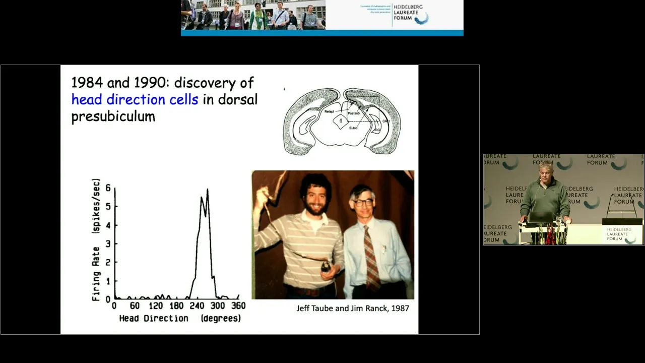
[00:07:41]And the third diagram is simply taking diagram B, which tracks where a cell fired, and normalizing it by the amount of time that the rat spent in each part of the environment. And that provides a sort of normalized firing plot showing you where that particular cell in the rat's brain would fire and where it wouldn't. And you can see it's still located just in that top right area of the environment. And that's why it's called a place cell. It represents a particular place in the environment. A few years later, the scientists also discovered a different type of cell called a head direction cell. And a head direction cell is a cell in the rat's brain that only fires when the head of the rat is facing in a particular direction. So for instance, there might be a head direction cell that only fires when the rat is facing facing in a northwards facing direction.

[00:08:41]Uh these little plots at the bottom sort of represent us an abstract representation of how much a cell would fire when the rat was facing in a certain orientation. So the distance of the thick black line from the origin represents the amount of firing or the firing rate of the cell for that particular direction. So for instance the plot at the far left is for a cell which would only fire when the rat was facing I guess in this diagram to the left or you could say in an absolute reference frame only firing when the rat was facing west. uh and it wouldn't fire very much at all when the rat was facing in any other direction. So this was known as a head direction cell and this is very exciting because this was another type of cell which is potentially very useful for tasks such as navigation.

[00:09:37]So by the 1980s approximately the scientists had found these two very interesting types of cell a place cell and a head direction cell. And they've done a lot of different experiments to sort of learn a bit more about how these cells behaved. And what they worked out was that the population of cells, so not just individual cells, but all the cells together maintain some sort of code or representation that described the rat's location and the rat's orientation, which we refer to as pose. So if you looked at the firing of all of the cells together, you could decode that the rat was located in a certain position and that its head was facing in a certain orientation.

[00:10:22]Now, if you took away some of the sensory input that the rat had, so for instance, if you turned out the lights, under certain conditions, the rat would continue to update which cells were firing based on its movement around the arena. So, even though the rat couldn't necessarily see where it was, it was still able to change how these cells were firing based on its movement through the environment.

[00:10:49]And this movement information came from senses such as the movement of the rat's legs and also from uh vestibular or acceleration sensors uh that the rat the rat has and indeed we have uh in our ear systems. The system was also worked out to also reset the firing of the cells based on distinctive visual input. So what that means was if the rat uh was wandering around for a while and then it was able to suddenly see a very distinctive visual landmark, something really clear and easy to understand, it could very rapidly change which particular cells were firing. So it had a way of based on on sensory input a way of quickly correcting or recalibrating its estimate of where it was in the environment by changing how these populations of cells were firing.

[00:11:45]So as roboticists who were very much coming from an engineering background, uh we tried to draw a diagram of how all these different parts of the rat brain which were thought to be involved at least somewhat with navigation were connected. And this was one of many different diagrams that we came up with because of course no one knows everything about how the brain works. Uh there's still a lot of unknown information. So everything isn't crystal clear necessarily. So this was one of our diagrams and first of all you can see that there are lots and lots of modules, lots and lots of different parts of the brain, lots and lots of connectivity. Uh the connectivity in this diagram is probably very far from correct but it was just one possible interpretation.

[00:12:30]uh and even this diagram is very much a simplification because each of these boxes represents a very complex part of the brain or very complex set of sensory inputs. So even this diagram is a gross simplification. Uh but to people just starting out in this field trying to create a model uh this was quite a daunting diagram. It looked very complicated.

[00:12:53]So in order to maintain our sanity so to speak, we simplified the diagram uh quite a bit. Uh and this is the system that we came up with. So we kept the place cells which represent the rat's location in the environment and we kept the head direction cells which represent the orientation of the rat's head. We had two types of input to our system. So this is this is rat slam version one. We had some sort of external landmark or visual input and this fed into both the place cells and the head direction cells. And we also had some form of selfm motion information feeding into the system. For a rat, this selfmotion information might come from the movement of its legs. For a robot with wheels, this motion information might come from the encoders on the wheels of the robot, which count how many times the wheels have gone around. And of course, there's no point creating a map of an environment unless you do something useful with that map. So, we wanted to use the output from this system to generate some sort of useful action such as navigating around the environment. So, to model uh all the different types of cells in our network, we needed some form of network that we could use. So back then we used what was one of the state-of-the-art ways of modeling these types of cells in the brain and we decided to use a continuous attractor network. So what I've got here is a simple schematic representing how you would use a continuous attractor network to model the head direction cells which represent the the orientation of the rat's head or in our case the orientation of the robot.

[00:14:37]So what I'll do here is unwrap that network. Uh but you could see it's in it in its original form. What we've done is we've associated each of these cells with a preferred orientation of the robot. So for instance, the cell at the far left uh was involved with representing the robot when it was facing at an angle of 180°. But for clarity sake, we'll just unwrap it into this straight line of cells.

[00:15:06]So a continuous attractor network is a special type of network that has a certain set of connections between the cells. First of all, cells are connected to nearby cells by excitatory or positive or reinforcing connections. So these connections allow activity or energy in the central cell to propagate or spread out to nearby cells. So they're positive cells. they help spread energy or activity in this network. There are also inhibitory connections from each cell to every single other cell in the network. And what happens there is that if cell the cell representing an orientation of 120° is activated, then it will inhibit or decrease the activity in all the other cells in the network by a certain amount through these inhibitory connections.

[00:16:05]Now I've only drawn in the previous slide the connections for one particular cell but if you draw all the connections simultaneously you can see that there is quite dense connectivity. So there are a lot of connections uh in this network but obviously it becomes very hard to visualize uh if you draw them all at once. Now, one of the fantastic things about these continuous attractor networks is that they have very specific dynamics, the sort of evolution of how active units will behave over time. So, what we're starting with here is an illustrative example where the unit representing a robot orientation of 60° is strongly active, represented by this blue rectangle. And the unit representing a robot orientation of 210° is also active. Not so strongly active, but but reasonably active. So, what happens when you let the the dynamics of the network unfold over time? Well, this is what happens. So you can see immediately that the activity spreads out from the central cell and then one cell tends to dominate. So we saw here if we go back we saw that the cell which started off with more energy first of all it spread the activity or energy outwards and then it eventually killed the energy in the other cell like so. And the stable state of this network in the absence of any more input or any more disturbances is this sort of peak of activity. So a cluster of units which are active with no other units active. And we refer to this as an activity packet or a packet of activity or an activity bump. There's a lot of different ways of referring to it, but this is the stable state of the network.

[00:18:00]Now we're using this continuous attractor network representing the head direction cells. We're using this network to represent the orientation of the robot. So what happens if the robot rotates on the spot? Well, it's going to change its orientation. It's going to change which direction it's facing. So you need a mechanism in this network to shift where the active cells are to represent the fact that a robot is rotating. So what you can do is use some form of selfm motion information and use connections once again some more connections in the network to shift the activity or shift the activity packet sideways to represent the robot rotating. So in this example we have the robot is currently encoded as facing in a direction of 120°. We can use these connections to shift or inject the activity to the side of these current cells in order to shift it around. So this is representing the robot turning from 120° to turning to something more like 135°. So this is the mechanism by which you can update your estimate of where the robot is facing or facing towards. And of course, if the robot turns back the other way, you can use another set of units, sorry, another set of links to shift the activity back the other way to represent rotation in the opposite direction. We also have another module in the rat slam system called the local view or LV for short. And you can see a diagram of the LV uh here in association with this head direction network. So the local view is a system which consists of a whole number of local view or LV cells represented by that little circle with an LV in it. So that represents one local view cell and each of these local view cells is associated with a distinct visual scene or a distinct visual landmark in the environment.

[00:20:12]So over time as the robot moves around the environment, it will learn a lot of local view cells because there will be lots of distinct visual scenes that it will see in the environment. And what happens is that each of these local view cells becomes associated with a particular set of head direction cells that were active at the time the robot saw that particular visual scene.

[00:20:39]So using one local view cell as an example, at a particular moment in time, the robot might see a distinct visual scene associated with that local view cell, what will happen is that the currently active head direction units, which might be the units representing an orientation of 120°, there will be connections between that local view cell and those particular head direction cells that will be strengthened at that time using a simple learning algorithm.

[00:21:10]And this is how the robot remembers which orientation it was facing when it saw that particular visual scene. Now, after a while, the robot might have wandered around quite a bit.

[00:21:21]Uh, and it might be thinking or estimating that it's facing in a different orientation, and that might be an orientation of 240°. So, this is a little later on time. The robots's wandered around and it it thinks it's facing in a direction of 240 degrees, but then it sees that visual scene that it remembers from before. And what happens is that local view unit or cell fires up and through those strengthened connections, it will inject activity into the head direction cells that it remembers it was that it remembers were active when it last saw that visual scene.

[00:22:03]And if it sees enough visual evidence, it will inject enough activity into those alternative head direction units in order to change the activity state of the head direction network. So what in effect this process is is a way of using visual scenes or visual landmarks to recorrect or reestimate which orientation the robot is facing it or in other words it's a way of calibrating uh where the robot thinks it's facing. Now what I've just presented was a onedimensional network. It only represented the orientation of the robot using this head direction network. We also had another population of cells in our model called the place cells. And the place cells in rats represent the location of the rat. And the location is actually a two-dimensional variable because it represents where the rat is over a flat two-dimensional surface. So, this is a two-dimensional version of a continuous attractor network. So, you're looking at a 144 units or cells laid out in a square grid and the colored patch is showing some of the units which are currently strongly active. So, you can imagine this square grid as almost representing say a floor plan and the currently active units are representing that the robot is perhaps at that location. You can use the same processes of shifting where the active units are around. So this is performing a process of path integration or motion integration by shifting the activity around in the network. So exactly the same as what we did previously but in two dimensions. You can also, if the robot sees a familiar visual scene or v familiar visual landmark, you can also inject activity into this cell network to represent the fact that the robot thinks it's back somewhere that it saw that scene before. And that's what's happening here. So the dominant packet of energy has switched from one location in the network to another location to represent the robot seeing a familiar visual scene.

[00:24:26]Now, there is one problem with this two-dimensional place cell network in that if the rat or the robot keeps heading in one direction for a very very long period of time, the activity or cluster of energy in the network is eventually going to hit one of the boundaries uh of that layout of neurons or units. And one way to solve this uh which has been come up come up with by quite a few people is to use wrapping connectivity in your network. So what you do is you connect the cells from on one boundary of your network all the way back to cells on the opposite boundary of your network. And what this does in effect is causes activity or a cluster of activity when it hits one boundary of the network, it will wrap around or circle around and re-enter on the opposite side. Uh and that means that the activity will never disappear off the edge. It will just come back on the other side. So this is one of the common ways of solving this problem.

[00:25:33]So once you've implemented this wrapping connectivity in your play cell network to solve this boundary problem, you can actually do some recordings of these artificial cells to see how they behave.

[00:25:45]So this diagram shows the recording from one particular cell as a virtual robot moved around a square arena. So, it's as if we're looking down on a square arena from on top and we're looking at where in the arena that particular cell fired.

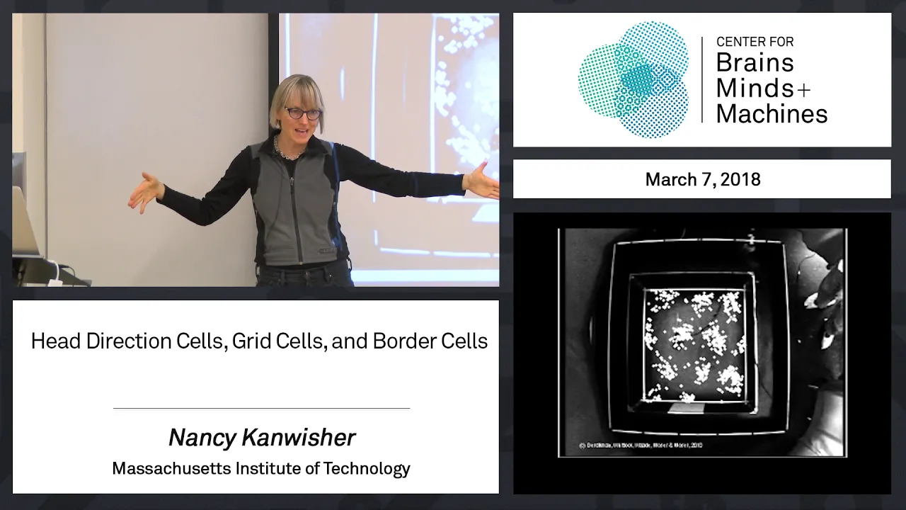
[00:26:03]And what you can see is that it fired at every one of a regular set of locations set out over a grid. So each of those clusters of color represent a location in this square environment where that particular cell would fire. And the reason it's firing at multiple locations in the environment is because of the wrapping connectivity that we discussed in the last slide. And this characteristic of a cell is actually quite similar to a relatively recent type of cell which has been discovered in the rat brain and also in many other animal brains.

[00:26:41]So, as I said, the whole methodology in this project was to start at the biology and then try and get a system working on a robot and then analyze how well the system worked, where it failed, and then go back to the biology to try and find some answers. So, back in 2003, we started running our first experiments.

[00:27:01]And these were quite simple experiments at the time. Uh we had a Pioneer 2 robot uh moving around in a 2x 2 m arena and it could see these artificial landmarks, these colored cylinders. And what we wanted to do simply was track whether the robot could maintain an accurate estimate of where it was inside this 2x2 m arena over a period of time. And the results that we found were actually a little surprising. So this is a graph of the error in the robot's estimate of where it was in the environment. And this is the estimate it obtained by using its place cell network and its head direction network. And time is along the horizontal x-axis. And you can see that over the first 10 or 20 minutes, the average error was maintained at about probably half a meter, a little less under half a meter.

[00:27:59]But over a longer period of time, the error grew and grew and grew until the error in where it thought it was in the environment was actually bigger than the 2x2 m arena it was supposed to stay in.

[00:28:12]So this was a surprising result. The system just didn't work. So we had to go back and look at the the cells as they fired over the entire experiment and do a lot of analysis and we were able to find out or identify a reason why the system failed. So this animation illustrates the failure mode illustrates the reason why the system wasn't able to maintain an accurate estimate of where it was.

[00:28:40]So, this is a mockup of the robot. We're once again looking from on high, looking from overhead, and it's in this environment where it's seeing a green cylinder. So, it sees a green cylinder, and it will have a certain number of place cells firing at that moment in time, representing that location in the environment where the robot is. And that's represented by that sort of green fuzzy patch on the left side of the slide. At the same time, it will also have some head direction cells firing that represent the fact that the robot is facing upwards or we're going to use the compass directions representing the fact that the robot is facing north. And that's what that graph at the right represents. It has a cluster of head direction cells that are firing representing the northward-f facing orientation of the robot.

[00:29:34]Now, at some later point in time, the robot might encounter this green cylinder again, but from a different orientation. So, in this case, the robot's come in from the right at the top, and it sees the green cylinder again. Now, it will have a different set of place cells representing that very different location in the environment.

[00:29:56]So, there's another patch of green fuzz representing the place cells that are firing for that other location. And it will also have another bunch of head direction cells representing the now westward or leftward facing direction of the robot. Then a little later on in time, the robot might come back and I'm not going to show you where the robot is, but all we're going to think about is what the robot can see. So the robot comes back at some stage and it can see a green cylinder again. Now it can see a green cylinder. So it says, well, there are two places I could be. And it activates the place cells representing those two possible locations. And that's what those two red patches represent. At the same time, it goes, well, there are two orientations I could be facing. I could be facing northwards or I could be facing westwards. And so it activates head direction cells representing those two possible orientations. And that's all very fine. That's representing all the possible locations and orientations the robot could be facing and where it could be located. The problem is as the robot wherever it is moves closer towards the green cylinder, you have a challenge of how can you can update your estimates of where you are in the environment. And the challenge pretty much comes down to you do not know which of the location hypotheses represented by the two red patches. You don't know which one of those goes with which one of the orientation estimates represented by that graph at the right showing both the northward facing and the westward facing estimate. So you have this sort of binding problem. You don't know which estimate goes with the other one. So, one of the only options you could do is have both orientation estimates associated with both place estimates.

[00:31:56]But that causes all sorts of problems because when you try and update your estimate of where you are based on the robot moving forward, you have this confusion because you don't know which orientation estimate to move your estimate of location along. So, you get all sorts of problems. This is just one of many possible failure modes that could result just illustrated schematically, but it it's illustrative of the basic problem. If however, and this is what we thought about at the time, you were able to somehow work out which one of the orientation estimates goes with each one of the location estimates. you'd actually be able to sens sensibly and independently update both estimates as the robot moved further forward. So, this is an animation showing what would happen in that case. And you can see that you can move both estimates in the correct direction. Uh, and they're still very sensible. And you could keep on updating them until you maybe saw another visual landmark which disambiguated or told you which one of your estimates was correct.

[00:33:10]So we learned from this work that unbound representations of direction and location or place can't be used when data as is ambiguous or when the landmarks are ambiguous and you need to track multiple hypotheses about where you could be and which direction you could be facing. Now we had a look back at the biology. So this is once again going back to biology to try and solve our problems. And this was back in 2003. So there was some very funky things you could do with phase synchrony or the timing of when neurons fire which might have been able to offer a potential solution. But there was a much more attractive solution which was to use conjunctive cells. And and what we mean by conjunctive cells was to invent a new type of cell which represented both orientation and location at the same time. And this would enable us to sensibly represent multiple hypotheses about where the robot was in the environment and which direction it was facing until we received sufficient evidence to work out which of these hypotheses was correct. uh and there's a much more recent publication uh in POS computational biology that you can read uh if you'd like some further information on this work. So this is when we moved on to the second version of rat slam. So what you're seeing in this slide is the first version which had the place cells and the head direction cells which is already a radical simplification of the underlying biology.

[00:34:46]So for this next version of rat slam, we combine the place cells and the head direction cells together to form a new type of cell called a pose cell. So it's exactly the same diagram as before except the two types of cells have been combined into one new type of cell. And this is what the pose cells look like.

[00:35:10]So this is a three-dimensional continuous attractor network representing this new type of cell called a pose cell or in this case it's the pose cell network. You can see that the network is laid out in three dimensions sort of like a rectangular or cubic cube rectangular prism or cube and each of the three axes of this prism roughly corresponds to one of the state variables of the robot. So we have x and y corresponding to the location of the robot and we have theta corresponding to the orientation of the robot. And like the head direction and play cell networks the stable state of the network is a cluster of active cells called an activity packet which is illustrated at the top right and this is published in our 2004 uh international conference on robotics and automation paper.

[00:36:06]This video shows the post cell network in action. The green blob that you can see, those are the currently active post cells. And the activity is going to shift around in the network based on motion information from the robot's wheels. So if the cluster of green moves up or down along the theta axis, that represents the robot rotating. If the act the cluster of green moves from side to side that represents the robot shifting along the ground. Now the robot can also see a familiar visual scene and inject activity into the network at a different location to represent the last place it saw that visual scene. And that's what just happened in that animation there. So about a year or two after we'd engineered this post cell to solve all our functional problems, there was a major discovery announced uh in neuroscience which was the discovery of a new type of cell called a grid cell.

[00:37:06]Now a grid cell is similar to a place cell except instead of the cell representing just one location in the environment, it actually represents any one of a number of locations laid out over a regular grid of locations throughout the environment. So this is a plot of the trajectory of a rat over a square arena over a long period of time.

[00:37:31]And everywhere that there's a red dot is where one particular cell fired. So you can see that instead of like a place cell where firing is restricted to one location, this cell is firing at a number of locations and that the arrangement of these locations is sort of laid out in a grid. Hence the name grid cell.

[00:37:57]Then shortly after that, they found grid cells in a deeper part of the brain which didn't just fire when the rat was at any one of a number of these locations, but also required the rat to be facing in a certain orientation. So these are known as conjunctive grid cells. They'll cells that fire only when the combination of rat location and rat orientation is appropriate for that particular cell. So in many respects they're very similar to post cells. And to actually investigate the similarity between the two types of cells, we actually went back and redid just about all of the experiments in that initial uh nature of science paper using the rat slam system. And we are able to show that with very minimal modification, the post cells in the rat slam system behaved remarkably similarly to the grid cells that had been discovered in rats. And there is a POS computational biology paper from 2010 with those results and much more in it.

[00:39:07]So going back to the overall diagram of the rat slam version two system, I'll talk a little bit about the types of input that we use and the processing algorithms uh that were deployed for this system. So first of all the landmark cues or really what this is is the visual input to the system.

[00:39:26]So this system works by looking at the current scene that the robot could see and this is a very sort of abstract representation of the scene that a robot might see and it would compare that scene to everything it had learned previously about the environment. So the robot would keep a library or a database of all the scenes it had ever seen and it would compare the current scene using some comparison metric to all these scenes that it had seen before. And if the scene was close enough to something it had seen before, it would activate or energize the local view cell associated with that visual scene. And this would in in turn activate pose cells which had last been active when the robot saw that visual scene. So that's its way of correcting or recalibrating its estimate of where the robot is in the environment. But of course, not every visual scene that it saw would be able to be recognized. Sometimes the robot would stray into a new unexplored part of the environment. So then it might see a scene which did not match to any of the current scenes. So would it add this scene to its library or its database uh learn a new local view cell associated with this new visual scene and it would also strengthen connections between that local view cell and the currently active post cells. So what it's doing in effect is remembering where it was when it saw that visual scene. So armed with rat slam version 2 complete with this new type of cell called the pose cells, we went back to do some more robot experiments. Now the initial experiments in the 2x2 m arena were quite successful. So interested in pushing the boundaries on how big an environment we could map, we scaled an experiment up to sort of half of a building floor. And we were able to form a a map uh represented by this colored shaded plot at the bottom right. And this is actually a temporal map showing navigation times between a place. So at the top left you can see the floor plan of the environment we were doing tests in including the robots path represented by the blue line. And at the bottom right you can see the corresponding map formed by the post cell system. And what we're doing in this particular experiment is using the temporal map formed to work out how to navigate between places. In this case, navigating from the bottom right part of the environment to the middle part of the environment. And we were able to perform some initial navigation experiments. And this was published in our 2005 international conference on robotics and automation paper. So encouraged by our successes uh in that initial environment, we expanded the environment size even more. So this is about double that environment size and we ran some experiments over a much longer period of time uh trying to do effective navigation between points. Now when we did this experiment in this larger environment over a longer period of time of 1 to 2 hours, we found that once again the robot was unable to navigate successfully. So once again we had a failure event and this is all part of this rinse and repeat process of looking at the biology creating a model testing it on a robot and then analyzing why it failed. So the particular graph that was most uh illustrative in demonstrating why the system wouldn't work in this new experiment uh is the one shown at the bottom right. So if over the course of an entire experiment you were to look down from up on above at the post cell network and track the location of the biggest or most dominant cluster of active cells over the entire experiment and plot a green dot uh on a graph for every uh second of the experiment you'd get the graph at or the figure at the bottom right. So every green dot represents where the dominant activity packet was in the XY plane of the post cell network. Now the black dashed lines represent relocization or recalibration events. So these were situations in which the robot saw a distinct visual scene uh and started to inject activity into the network that was somewhere very different to where the current dominant activity packet was. And with enough visual evidence, that location where it was injecting activity would actually form its own activity packet which would eventually become dominant. And so that was the the method by which we could recalibrate or recorrect errors that might have built up over time based on the wheels slipping on the carpet and other factors like that. The implication of this is that there are lots of discontinuities uh in this postell network. So the layout of the postell network which initially represented quite nicely the xy layout of the environment uh initi rapidly becomes uh less and less representative of the actual physical layout of the building floor or the office building floor because of all these discontinuities. And the end effect of this is that you can no longer interpret the post cell network as representing directly the physical layout or physical structure of the environment. And if you can't do that, you can't navigate very effectively. And this is why our system was failing again. So we went back to the drawing board and redesigned Rat Slam version 3.

[00:45:08]And this is the pretty much the final version of Rat Slam. and the mature version as it is today. So what's shown at the moment is rat slam version two.

[00:45:17]What we did is we added an extra model or module called the experience map. And the experience map's role was amongst other things to take this very dis discontinuous representation of space in the post cells and create a much more continuous much more usable map that the robot and indeed a human could actually use to perform useful things like navigation. So this is a schematic of the third version of rat slam. So at the top left we have the local view cells.

[00:45:52]Each one of these cells represents a distinct visual scene. And this is what you've seen in the past slides. At the bottom left, we have this three-dimensional continuous attractor network representing the pose cells. And this is the robot's internal estimate of the robot's location and orientation in the environment, but a representation which becomes very discontinuous over time. As you saw in the previous slides, the output from both the local view cell network and the post cell network is used to form a new map called an experience map. And that's what's shown at the right of the slide. And the experience map is made up of nodes or experiences represented by the black circles representing distinct places and scenes in the environment. And as the robot would move around, it would form more and more of these experiences or nodes. And each of these experiences would be connected by transitions or connections representing the the movement from one place to the next. And essentially you would learn a new node or new experience in the map whenever none of the current nodes or experiences in the map matched closely enough to the current state in the local view cells and the pose cells. So whenever you saw a went to a new place or saw a new distinct visual scene, you would learn a new experience or place. So in a little more detail, this is what the experience map looks like.

[00:47:26]There's an example experience map at the right with a little zoomed on inset and each of the little green circles represents an experience or node in the map connected by transitions represented by the blue line between the experiences. The experience map is is semimetric. So its layout in space is meant to roughly correspond to the actual physical layout of the environment that the robot's moving through. it won't necessarily be accurate uh to the nearest millimeter. Uh one it has many many benefits apart from generating a map which looks uh much easier for a human to interpret uh the experience map also removes aliasing of landmark cues. So what in effect this means is that if you have some visual scenes in the environment or places in the environment which look the same even though they're quite different places uh the experience map helps you disambiguate uh these two places. So in order to make the map represent the layout of the environment as much as possible we continuously form a perform a process called graph relaxation on this experience map. So if we have a robot which has learned a place represented by that green circle and it moves around and it goes to a new place learns that place which is a second green circle as well as a transition between those places. Uh this is how it builds up its experience map and this process will continue until it's completed the loop and it's come back to the very start uh where it first started off. Now, because of errors, perhaps the wheels slipped slightly on the carpet or or because of other factors, the robot's estimate of where it is in space might be slightly different to the beginning of the loop.

[00:49:11]It there might be a slight discrepancy there. But because the robot has a camera, it can see that it's back where it started. So, there's a there's a discrepancy or disagreement between where its camera says it is and where its updated estimate of location thinks it is. And that's represented by the difference between the dashed circle and the original circle. So what graph relaxation does is it averages those two uh pieces of information and distributes any errors or discrepancies evenly around the entire graphical network. So you can see here that the network's shifting around uh until it reaches a stable state. And that's what graph relaxation is.

[00:49:57]Another useful characteristic of the experience map is that you can perform a process called map pruning. So this is an abstract representation of a simple experience map with six places that the system seven places that the system has learned. Now, if you're performing experiments over very long periods of time, uh you don't want to keep learning more and more places because eventually your computer won't be able to store them all or it won't be able to compute where it is fast enough in order for the robot to work. So, you can perform a process such as map pruning to help maintain a reasonable number of places in the map. So, for instance, you can divide your experience map up into a grid and make sure that there's never more than one place represented in any one of these grid squares. So, if you've got two, like in this example, you would delete one and reconnect the other. And that way, you'd keep the number of nodes or places to a manageable number over time. Another useful thing you can do with an experience map or graphical map is perform processes like path planning.

[00:51:03]So planning a path from where you are now to a goal. So as well as storing nodes or places represented by the green circles, the experience map also stores transitions represented by the blue lines. And these represent movement between places. And these transitions can store a number of pieces of information. They can store distance information, speed information, or even temporal information, how long it takes to get from one place to another. And you can use this temporal information to plan the quickest route between two places. So this is an example of trying to find a route from the start location marked at the far right of the map to the goal location. And by there's always one unique path which is the fastest route to the end location based on the time intervals between each of these nodes. And you can use that to actually plan and then execute the fastest path to a goal. So this is an example of the whole system in action. You've seen the pose cells at the top left before, but what you're seeing now is the experience map at the bottom uh as it's formed, as the robot moves around the environment and as it warps around. That's the graph relaxation algorithm at work. And at the right you can see the unique ID or number of each of the visual scenes in the environment. So each visual scene that the robot sees is associated with a a number or a local view cell number.

[00:52:34]And when the robot comes back to a place it's been before, it might recognize some visual scenes from that place. And that's when the number will jump back to a much smaller number such as 6 or 50.

[00:52:45]That's the system recognizing a place that it's been before. After a few seconds, uh the map that's formed of the environment is quite stable.

[00:52:55]So now that you've seen the rat slam system or the mature version three of the ratlam system, I'm going to talk about the two experiments or two of the major experiments that we performed with this system. The first of these was an experiment where we set out to map an entire suburb of Brisbane, my hometown, using just the web camera in a MacBook computer. So this is an overhead view of the suburb showing pretty much every road that we drove along. Uh it was about 66 km of driving uh in a period of time just under 2 hours. You can see my old car there with the computer strapped to the top and all we were doing was recording from the webcam. And this is a webcam from back from 2007208. So the quality wasn't as great as it was today. And the idea was to try and create a map of this entire system without using any other sensory inputs.

[00:53:50]So no GPS, no speed from the wheel encoders, no steering angle from the steering wheel, nothing like that. Just using the camera feed. Now the rat slam system, as shown in those diagrams before, it needs two types of input. It needs some type of selfm motion information input. So it needs to be able to work out how fast it's moving and how much the vehicle or the robot is rotating. So to calculate this, what we did is we used a remarkably simple system. So this at the top left there's an image from the webcam. So we took a subframe of this shown by the blue rectangle and what we did is we summed the intensity values of the pixels in each column of that blue rectangle. And that gave us what we call an intensity profile. And that's represented on the top right figure on this slide. So what you're seeing there is actually two intensity profiles from consecutive frames. So from frames one after the other. Now to detect how much the vehicle was rotating, what we did is we compared these consecutive intensity profiles to each other over a range of relative offsets. So what we did is we shifted one relative to the other to see for which relative shift they matched the most closely and that generated a difference plot which is the bottom right figure showing you how closely the two intensity profiles matched for different relative offsets. And you can see that the smallest difference was for an offset of about 70°. And so this offset was what we used to work out our rotational velocity. So it's simply just shifting or looking at how much the image shifts from one side to the other to get a crude estimate of the rotational velocity of the vehicle.

[00:55:45]Now we still needed to get an estimate of how fast the vehicle was moving. So the translational velocity of the vehicle and we did this simply by taking the minimum difference score. So you can see in the bottom right figure for the best matching relative offsets, the difference is still about two 2.2 or something like that. So we use that measure as a simple measure of speed. We call it perceptual speed. Uh it's it's quite crude, but it seemed to work well enough uh in this experiment. So this is the video of the actual experiment. At the top left, you can see the video feed from the web camera in the laptop. uh as the car drove around the environment. At the top right, you can see a reference map of the environment we were mapping. So, this is shown in red, all the roads that we drove around. And at the bottom, you can see the experience map. So, I'm not showing you any of the neural networks or any of that. I'm just showing you the output, the experience map. So, as the car turns around the corner, you can see the experience map uh represents the curve reasonably well. And what's going to happen is the video is going to speed up shortly.

[00:56:55]So you don't have to sit through uh 2 hours of experiment. But what's happening here is we're getting back to the start of a 5 km loop and the system is able to recognize that it's back where it started, join those two parts of the map together and then the graph relaxation process smooths out the map until it forms a stable state. So this is a second loop of the environment that we're doing here. So we're in the aerial photo, we're in the bottom right section of the environment.

[00:57:25]And so we're still moving around and you can see a second loop that we're just about to finish. And you can see the map warping around to represent corrections.

[00:57:34]And a third loop here. And a fourth loop. And then another major loop closure here. So you can see that the system is correcting for quite major errors that accumulate because the velocity estimation system that we're using is relatively primitive. uh it's not particularly sophisticated, but you can see we're still able to generate quite a good map uh using this system. So, if you look at the map at the top right and the map, the experience map, you can see that they already correspond uh reasonably well.

[00:58:07]And just to reemphasize, we're just using the input from the camera. We're not using GPS. Uh we're not using any other type of sensory information. We're not using the angle, steering angle of the wheels. We're just using uh this quite lowquality web camera. So, I'll just let the video run uh for now. Uh and you can watch the map unfold.

[00:58:49]So this is the experience map produced at the end of the experiment compared to the actual environment. So first of all you can see that it's quite a complex network of roads but it's represented uh quite faithfully by the experience map.

[00:59:02]The actual precise metric layout of the map isn't identical to the environment but the topology that is how the map is connected together is all correct and representative of the environment.

[00:59:17]This slide gives an example of the challenge that the system was solving.

[00:59:23]So everywhere on this map that you can see a red dot is somewhere where the vision system thought it was in the same place. So there are 42 different locations that the vision system thought were the same place. And it's only through the robust filtering of uncertainty that is provided by the post cell network and the experience map that the system is able to deal with this level of uncertainty and this level of ambiguity and create a coherent correct map.

[00:59:58]This is a zoomed up section showing you the experience map and showing you where along the route two particular sets of post cells fired. So everywhere that you see red dots, one particular set of post cells would fire. So as the car would move through the center of the firing field for that cell, it would the cell would fire more and more strongly represented by bigger red circles and then the firing rate or firing amount would drop off as the car moved out of the firing field. And this is vaguely analogous to the firing fields of actual grid cells in actual rats, although of course they're not tested in an environment like this.

[01:00:45]This was a second experiment that we performed using rat slam which was one of our major pieces of work published in the international journal of robotics research in 2010 known as the office delivery challenge. So we used a Pioneer 3 robot which you can see in that picture equipped with a panoramic camera. So this is a camera that looks upwards at a panoramic mirror allowing the robot to see in 360°.

[01:01:12]Uh, it also had a laser to help it stop hitting things, but all the mapping and navigation was done primarily using the camera. The encoders on the wheels provided the robot with an estimate of how fast it was moving, and it also had some ultrasound sensors to help it stop hitting things in addition to the laser.

[01:01:31]So, the challenge was we took the robot effectively out of a box into an unknown office and laboratory complex. Uh so the robot had no map when it started this experiment and it reverted to its default behavior which was to using uh its exploration behaviors forage around the entire environment and create a map.

[01:01:52]After a couple of hours of doing this, the robot had formed an experience map like you saw in the previous experiment and a human person assigned six delivery locations by clicking on the map on a computer. And these were locations that the robot had to pick at random and go to as if to make a mock delivery. So we ran this experiment over a period of about 1 and a half weeks uh where the robot would just randomly pick one of these delivery locations to navigate to. And it did this at all times of day and night. So he ran some of these experiments at 2:00 a.m. in the morning, some of them in the middle of a busy day. It also had to find its charging station. So, we told it what its charging station looked like, but we didn't tell it where it was in the environment. So, the robot, while exploring and navigating around, it had to keep an eye out for its charging station so that it could when necessary autonomously navigate back to the charging station and charge to top up its batteries. And so, this all happened over a period of 1 and 1/2 weeks completely autonomously with pretty much no human intervention.

[01:03:04]So to make the experiment a little more challenging, after the robot had returned to the charger and powered down for one of its recharge cycles, we took the robot across the across the road to another office building environment and turned it on without telling it anything about the fact its environment had changed. So the robot woke up, it started because it didn't recognize anything, it started to explore this new environment. uh and it continued not to recognize anything because this was a completely novel environment and it managed to form a map after about an hour and a half of this new environment. So, a human assigned five new delivery locations by clicking on locations in this new map. And it should be noted that we never explicitly told the robot it had changed environments.

[01:03:51]So, it still had its map of the previous environment entirely in memory. It was just that it wasn't able to recognize any of those locations because it was indeed in a different environment. So the robot started to make mock deliveries to these five locations and we let it perform I think 50 something deliveries in this new environment uh until it ran out of charge. It managed to locate its charging station which we'd moved across to the new building.

[01:04:18]Uh autonomously return to the charging station and recharge itself. Then without telling it once again, we kidnapped it back to the first office environment. Uh and once it had recharged, uh we turned it on again. It woke up. It moved around within a couple of seconds. It recognized it was back in the original environment. Uh localized or worked out where it was in the map and then immediately started making mock deliveries to the original six delivery locations. So it did a full cycle of I think about 70 deliveries in the original environment before it returned to the charging station to recharge and that was the end of the experiment. This slide presents the vision system used for this experiment.

[01:05:04]Overall, it was similar to the one used in the previous experiment, except that we are actually able to use panoramic 360 degree images obtained from the camera and mirror setup on the robot.

[01:05:16]So, the robot could see in 360° field of view. A human has a field of view of about 180° for reference, but that was essentially the vision system, and it used relatively low resolution versions of these images to try and recognize familiar places.

[01:05:33]and so forth. So, I mentioned before that the robot didn't actually use its sonar sensors or its laser sensor to perform mapping. What it did use these sensors for were to help it avoid hitting things and to help it move smoothly around obstacles. So, you can see one of the scenarios that the robot encountered uh quite late at night was encountering the janitor's car, which would be at a random position in the environment. So, it of course had to find its way around that. So the robot had a sophisticated system of what we call local movement behaviors which enabled it to a not hit things and b move smoothly around obstacles in the environment. And this was a critical part of the experiment running successfully over that period of 2 weeks. This is one of the uh results figures for the experiment. So what you can see here are the six delivery locations in the first environment and the five delivery locations in the second environment. The little black circle hollow circle is the designated delivery location that the robot was supposed to go to. Each of the gray squares was the location the robot actually went to when it went to make the delivery. And the little black dot at the middle of the gray crosses is the average or centrid of those gray crosses for each of the delivery locations. You can also see some gray crosses at the top right of the first figure which don't have a delivery location associated with them. So, that was the part of the environment where we put the charging station, and that was where the robot would navigate to before it would start a homing procedure to navigate over onto the charging dock, which you'll see in a video shortly, uh, and recharge. And it's interesting to note that the homing system for recharging was accurate to about 50 mm. So, we could position the robot at a location to within about 50 mm quite consistently. It had to, otherwise, it would have failed recharging. and the experiment would have failed. If we'd used one of those homing procedures at any all the other delivery locations, the performance would have been a lot more accurate. But this is performance was plenty accurate enough to demonstrate the basic concept. We were getting to within about a meter of the delivery location. Uh which was which was quite good. We thought this video shows what the robot saw every time it reached goal location number six in the environment. So this is a snapshot of that part of the environment every time the robot thought it had reached that location. So you can see first of all that sometimes it's nighttime, sometimes it's daytime by the brightness of the window. And you can also see that it's quite repeatable uh in that it's visiting pretty much exactly the same location each time. Uh and this occurred continuously over the two weeks. And you can obviously see uh this person that this poor person that we're constantly the robot is stopping next to. This is a video of an actual navigation trial during the experiment.

[01:08:42]One of the more than a thousand which occurred. So, the robot has just woken up from the charging station. It's picked a goal at the other end of the building to navigate to. So, it's formed a plan for reaching that location. It's navigating along that planned route. And when it gets to the location where it's supposed to form the the mock delivery, it doesn't actually do an actual delivery. It will log lots of data and say something.

[01:09:12]So that's it indicating that it thinks it's reached the delivery location. This video shows the progression of the experience map for the first environment over the course of the two weeks. So you can see that while it does warp around a little bit, the connectivity and the layout of the map still correctly represents the layout of the environment.

[01:09:37]One of the important pieces of analysis that we wanted to perform on the experiment or the experimental results was whether the system was stable over time. So this is a graph of the number of experiences. So the number of places that the map stored of the world and also the number of visual scenes that the system learned or had stored in memory at any one time. So you can see that over the first 32 active hours of active navigation and exploration of the experiment, the number of experiences and the number of visual templates stays roughly stable. And we have some more detailed analysis of the stability in the 2010 paper. And then it jumps at around the 32-hour mark because we've gone to a second environment and it's still storing the entire first environment in memory while also learning the second environment. But then once it's learned the second environment uh the number of experiences and the number of visual templates uh remained relatively stable at least over that short period of time and once again there's more detailed statistical analysis of the stability showing that it is stable to a significant level uh in the paper. This slide shows the delivery performance and also a summary statistic. So over the entire 2e experiment, the robot was called upon to perform 1178 navigation trials or delivery trials and it performed 1177 of those successfully. So it had a more than a 99.9% success rate. The only fail failure came uh when the robot became temporarily very badly lost uh and it was unable to reach one particular delivery location. The robot tried for a period of about five minutes before it timed out and then continued on its way and started delivering to the next location. So, it had a robust recovery from this single failure. And as of the making of this presentation, it's still one of the only robotic systems to perform continual mapping and navigation over a long period of time using vision as the primary modality.

[01:11:57]So after those two experiments and many other experiments which have been published over the last 10 years, we came to the conclusion that rodent biology can indeed form the basis for a robot navigation system which is at least competitive in some aspects with state-of-the-art mathematical or probabilistic based robot mapping and navigation techniques. But to achieve the sort of uh performance that we did, we had to pitch it at the right level.

[01:12:25]So we had to start with the biology. Uh where the biology couldn't provide answers to a problem, we had to adapt it or engineer a solution uh in order to progress to the next step. And then by closing the loop back to the biology, we're sometimes able to find that some of the engineered solutions might actually be relevant to the biology. So it is very much a closed loop process.

[01:12:50]You go from biology to robotics and then back again. And in our approach, we solved or addressed the robot mapping and navigation problem really as a learning and recall problem. So it would learn the association between places and visual scenes in the environment and then recall sequences of these places in order to perform navigation. And this is a very different approach to the approach which is pretty much geometric optimization of many of the more mathematicalbased robot slam or mapping systems. If this talk has got you a little bit interested in Rat Slam and you'd like to try it out yourself, we have an open-source version of RatSlam available at that link. And we have two versions, one integrated with the robot operating system Ross and one standalone C++ version. So you can download them, follow the instructions and run them on some data sets, perhaps even gather your own data sets or get them working, get Ratlam working on your own robot.

[01:13:58]The work done on this project was funded jointly by the Australian Research Council and the National Health and Medical Research Council of Australia at least partially through the thinking systems strategic research initiative and also by the Australian Research Council Discovery Project Scheme. And there are many thanks uh deserved thanks to all the colleagues who I've worked with over the years who've contributed to this project and in particular David Presser, Janet Wilds, David Ball, and Will Madden. Well, that brings us to the end of this video presentation. Hopefully throughout this talk I've managed to give you a bit of an overview of what rat slam is, what the rat slam system does, its basis or inspiration in rats and rat navigation, and also being able to present some of the more pivotal experiments that we performed over the years uh using rat slam. I'd like to thank you very much for coming along and watching my video. Uh if you have any questions, please feel free to leave a comment. Thanks for watching.