Building Ballbots: Dynamics, Kalman & LQR

Learning Goal: Design, build, and program a dynamically stable "Ballbot"—a robot balancing on a single sphere—using three omniwheels, an IMU for Kalman-filtered state estimation, and a state-space Linear Quadratic Regulator (LQR) control system on a Teensy microcontroller.

• Prerequisites: Basic understanding of Newtonian physics (forces, torques), linear algebra (vectors, matrices), and entry-level C++ programming (loops, variables, functions).
• Estimated Total Study Time: 42 Hours

---

Module 1: Embedded Electronics & Omniwheel Actuation

This module establishes the foundational hardware components of the Ballbot. You will learn to interface with the high-performance Teensy microcontroller, wire and configure DC motors with quadrature encoders for precise rotational feedback, and analyze the unique physics of omniwheels. These multi-directional wheels are the core mechanical elements that allow the robot to transfer torque to the balancing sphere across different axes.

Recommended Videos

Hardware Overview: Teensy Microcontrollers

Why this video is valuable: This video provides an excellent introduction to the Teensy development ecosystem, comparing its clock speed and hardware parameters with standard Arduino boards. To process complex Kalman state estimation and LQR matrix math in real-time, standard 8-bit microcontrollers (like the Arduino Uno) are insufficient. The 32-bit ARM Cortex-M architecture of the Teensy (running at 72MHz to 600MHz depending on the model) offers the hardware floating-point units (FPU) and memory footprint needed for this project.

Note for modern builds: While this video features the Teensy 3.2, current designs should utilize the Teensy 4.0 or 4.1. The programming workflow via the Teensyduino add-on for the Arduino IDE remains identical.

---

Initial Setup & Programming of Teensy

Why this video is valuable: This short, practical guide demonstrates how to configure the Teensy Loader software and link it to your programming environment. Understanding the uploading mechanism and physical button usage on the Teensy is essential before writing your first actuator control code.

---

Decoupling Omniwheel Physics

Why this video is valuable: James Bruton demystifies the mechanics of omnidirectional wheels. He explains how passive peripheral rollers allow the wheel to slide friction-free along its axial direction while transferring direct drive forces in its radial direction. Understanding this dual-velocity mechanism is critical for deriving the kinematic matrix that coordinates your three motor outputs into a unified sphere-driving force.

---

Closed-loop DC Motor Control & Quadrature Encoders

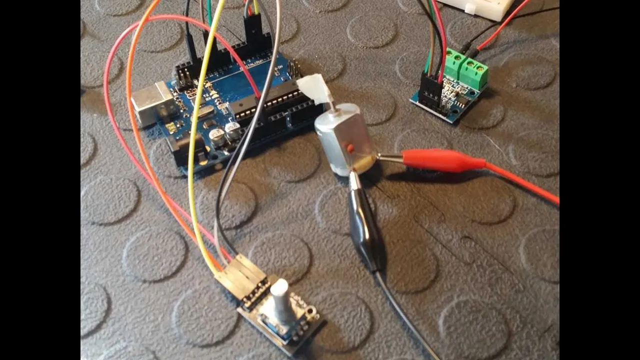
Why this video is valuable: To balance, your LQR controller needs precise motor velocity feedback. This tutorial covers wiring a dual-channel quadrature encoder to microcontroller interrupt pins. It explains how to interpret the phase-shifted A and B square-wave signals to determine both the direction and exact speed of the motor shafts.

---

Knowledge Checkpoint

• Write a non-blocking Teensy sketch that reads raw quadrature encoder pulses using hardware interrupts (attachInterrupt()).
• Calculate the angular velocity ($\omega$) of a motor shaft in radians per second given a CPR (Counts Per Revolution) value and loop timing.
• Draw a force diagram of a single omniwheel demonstrating where force is transferred (traction) versus where it is dissipated (passive rolling).
• Explain why a 32-bit ARM processor (Teensy) is required over an 8-bit AVR processor (Arduino Uno) for executing matrix algebra at high loop rates (e.g., $200\text{ Hz}$).

---

Module 2: Ballbot Kinematics & Rigid Body Dynamics

This module covers the core mathematical modeling of the Ballbot. You will study how forces translate from three omniwheels arranged at $120^\circ$ angles onto a single sphere, and use Lagrangian mechanics to derive the equations of motion for a 3D inverted pendulum.

Recommended Videos

Conceptual Ballbot Systems & Control Challenges

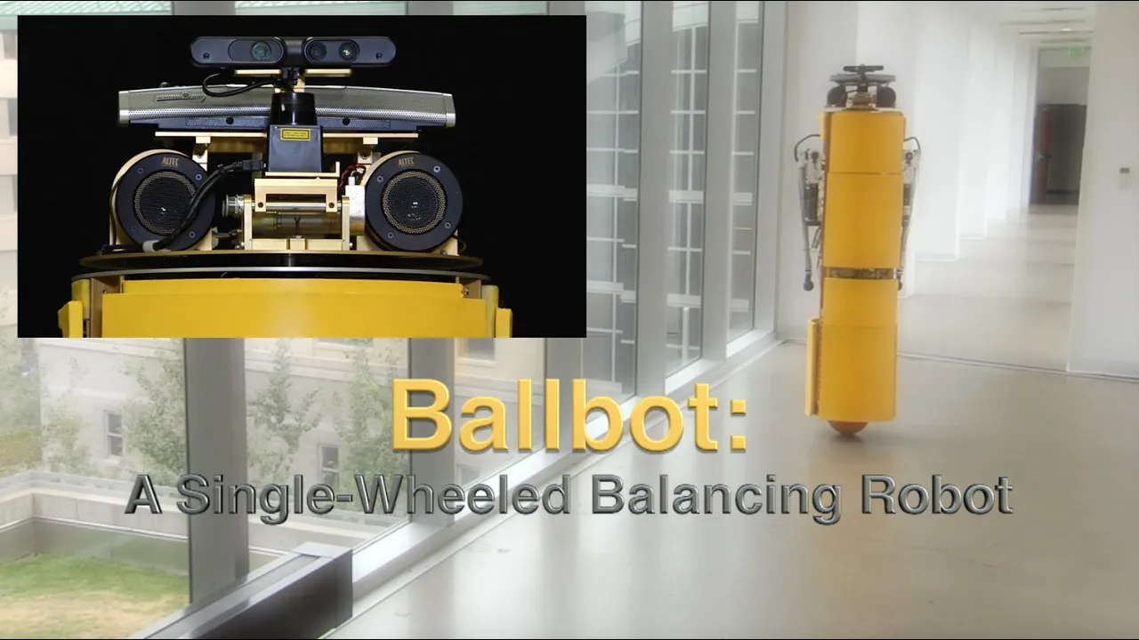
Why this video is valuable: This video from Carnegie Mellon University—the birthplace of the Ballbot—provides a clear overview of the robot's mechanical layout, structural dynamics, and operational envelope. It shows how the robot operates as an underactuated system, moving by intentionally falling in the direction of travel and catching itself using the rolling sphere.

---

Introduction to Lagrangian Mechanics

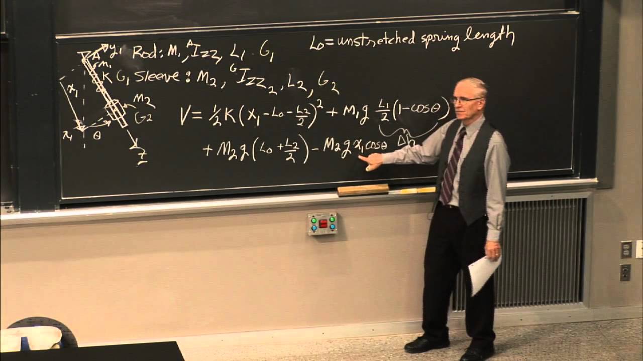
Why this video is valuable: To model a complex system like a 3D inverted pendulum, standard Newtonian force-balance equations ($F=ma$) quickly become unmanageable. This MIT lecture introduces Lagrangian mechanics, a energy-based method where the equations of motion are derived from the Lagrangian ($L = T - V$, kinetic energy minus potential energy).

---

Deriving Equations of Motion for an Inverted Pendulum

Why this video is valuable: This lecture applies the Euler-Lagrange equation to a classic inverted pendulum. This derivation serves as the direct mathematical template for modeling your Ballbot. The resulting non-linear differential equations will later be linearized around the vertical operating point to construct the LQR controller.

---

Practical Multiaxial Balancing Mechanics

Why this video is valuable: James Bruton walks through the construction and physical tuning of his own ball-balancing robot ("HAL9000"). This video provides practical context for the dynamics of multi-axis balancing, showing how misalignment, weight distribution, and sensor placement can introduce physical unbalances that must be addressed in your control software.

---

Kinematics Gap Fill: 3-Omniwheel Ball Kinematics

Because video coverage of the exact coordinate transformations for a three-omniwheel system driving a sphere is limited, use the following derivation for your code implementation:

Let the ball have radius $r_w$ and the omniwheels have radius $r_k$. The three omniwheels are arranged symmetrically at $120^\circ$ intervals around the top of the sphere, tilted at an angle $\alpha$ relative to the horizontal plane.

To convert the desired virtual sphere velocities (expressed as rotation rates $\omega_x, \omega_y, \omega_z$ about the robot's local frame) into individual motor target angular velocities ($\Omega_1, \Omega_2, \Omega_3$), we use the inverse kinematics transformation matrix:

$\begin{bmatrix} \Omega_1 \\ \Omega_2 \\ \Omega_3 \end{bmatrix} = \frac{r_w}{r_k} \begin{bmatrix} -\cos\alpha & 0 & \sin\alpha \\ \frac{1}{2}\cos\alpha & -\frac{\sqrt{3}}{2}\cos\alpha & \sin\alpha \\ \frac{1}{2}\cos\alpha & \frac{\sqrt{3}}{2}\cos\alpha & \sin\alpha \end{bmatrix} \begin{bmatrix} \omega_x \\ \omega_y \\ \omega_z \end{bmatrix}$

This matrix distributes the orthogonal control efforts computed by your LQR controller to the physically canted actuators.

Knowledge Checkpoint

• Define the Lagrangian $L$ for a simplified 2D cart-pendulum system and write out the Euler-Lagrange equations.
• State the physical meaning of "underactuated" system dynamics and how it applies to a Ballbot.
• Perform a coordinate rotation to project the robot's pitch ($\theta_x$) and roll ($\theta_y$) tilts into corresponding motion directions on the horizontal floor plane.
• Calculate individual motor velocities ($\Omega_1, \Omega_2, \Omega_3$) given a target sphere rotation of $\omega_x = 2.0\text{ rad/s}$ and $\omega_y = 0\text{ rad/s}$ using the kinematic matrix above.

---

Module 3: IMU Sensors & Kalman Filter State Estimation

To balance, the robot needs to know its exact orientation relative to the gravity vector in real-time. This module explains how Micro-Electro-Mechanical Systems (MEMS) accelerometers and gyroscopes operate, analyzes sensor noise, and shows how to combine their readings using a Kalman filter.

+-------------------------+ | State Transition Model | | (Prediction) | +------------+------------+ | | Predicted State (High-rate, drifts) v

+-----------------+ +----+----+ +-----------------+ | Gyroscope +------>+ Kalman +<------+ Accelerometer | | (Ang. Velocity)| | Filter | | (Linear Gravity)| +-----------------+ +----+----+ +-----------------+ | | Corrected State (No drift, low noise) v +------------+------------+ | True Tilt Angle | | State Estimate | +-------------------------+

Recommended Videos

Inside MEMS Accelerometers

Why this video is valuable: This high-speed microscope teardown shows the internal comb-like silicon structures of a MEMS accelerometer. You will see how physical acceleration deflects a micro-machined proof mass, changing its electrical capacitance. This sensor provides an absolute reference for the gravity vector, which is highly accurate at rest but corrupted by high-frequency vibration when the robot moves.

---

Inside MEMS Gyroscopes

Why this video is valuable: This animation shows the internal operation of a vibrating-structure gyroscope. It explains how the Coriolis effect deflects vibrating silicon elements when the chip rotates, generating a voltage proportional to angular velocity. Integrating this velocity yields highly accurate short-term tilt angles, but sensor bias causes this value to drift over time.

---

Intuitive Kalman Filter Theory

Why this video is valuable: This tutorial explains the math behind the Kalman filter without getting bogged down in notation. It shows how the algorithm balances a dynamic prediction (integrating the gyro) with a noisy measurement (the accelerometer reading) by calculating the "Kalman Gain" based on the relative uncertainty of each source.

---

C++ Sensor Fusion Implementation

Why this video is valuable: This video translates Kalman filter theory into direct, executable C++ code. It walks through setting up state matrices, covariance matrices, and executing the prediction and correction loop cycles. You can adapt this structure directly for your Teensy firmware.

---

Knowledge Checkpoint

• Explain why you cannot calculate tilt angles using only an accelerometer or only a gyroscope on a rolling robot.
• Identify the state vector ($x$), process noise covariance ($Q$), and measurement noise covariance ($R$) for a 1D tilt Kalman filter.
• Implement a C++ class that takes raw IMU variables ($a_x, a_y, a_z, g_x, g_y, g_z$) and outputs a filtered pitch ($\theta$) and roll ($\phi$) angle.
• Measure and calculate the bias drift of your gyroscope at rest, and explain how the Kalman filter compensates for this offset.

---

Module 4: State-Space Control & LQR Design

With your kinematics modeled and states estimated, you can now design the balancing controller. This module introduces state-space representation and explains how to design a Linear Quadratic Regulator (LQR) to calculate optimal control gains.

+-----------------------+ Feedback Gain K | LQR Controller |<-------------------------------+ | u = -K * x | | +-----------+-----------+ | | | | Control Effort (u) | v | +-----------+-----------+ | | Physical Ballbot | | | (Plant Dynamics) | | +-----------+-----------+ | | | | State Vector (x) | | [position, velocity, angle, ang_velocity] | +--------------------------------------------+

Recommended Videos

Introduction to State-Space Representation

Why this video is valuable: Classical control methods like PID focus on single-input, single-output (SISO) transfer functions. A Ballbot, however, is a multi-input, multi-output (MIMO) system. This video shows how to convert high-order differential equations into a state-space system of first-order matrix equations:

$\dot{x} = Ax + Bu$

$y = Cx + Du$

---

The LQR Optimization Framework

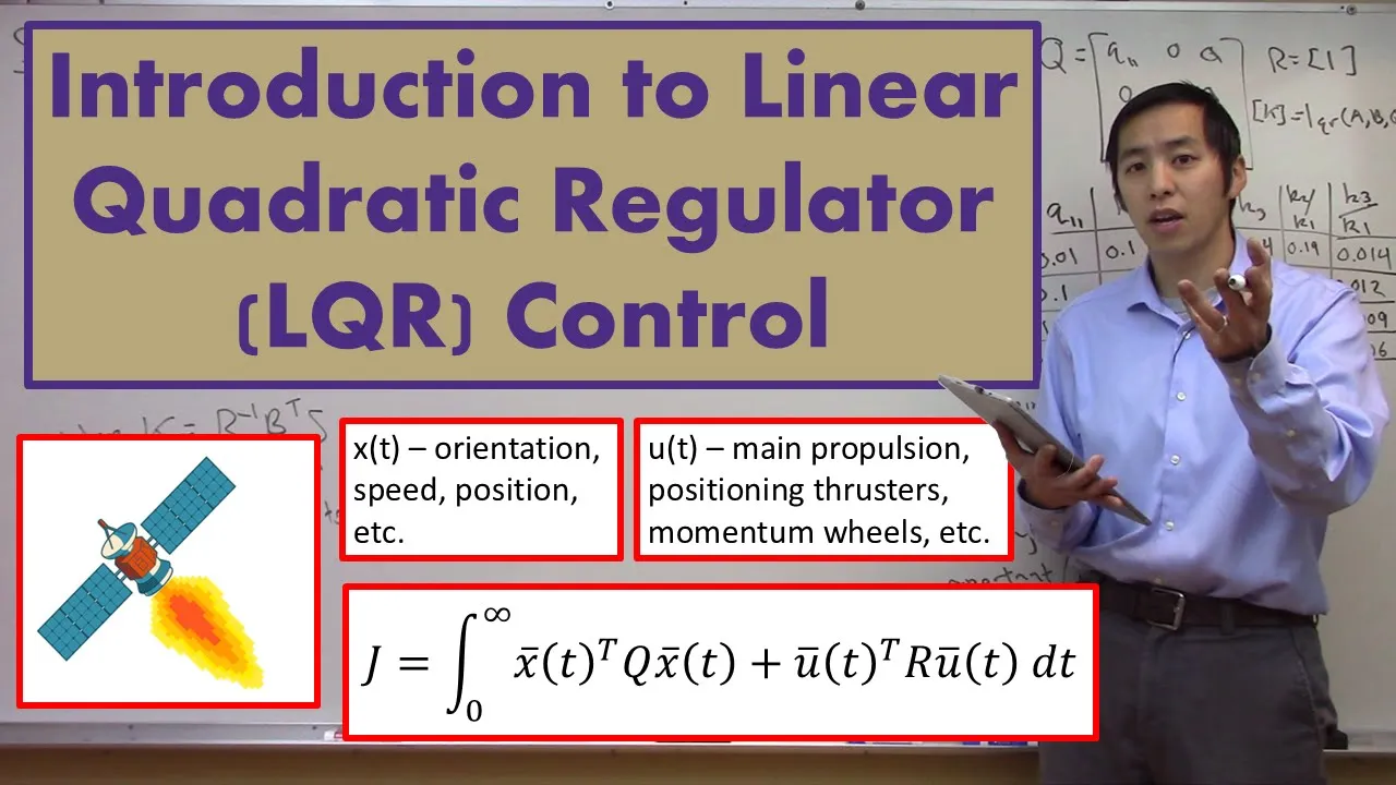
Why this video is valuable: Christopher Lum explains the mathematics of the Linear Quadratic Regulator. LQR calculates the optimal feedback gain matrix $K$ by solving a cost minimization problem that balances performance against actuator effort. This cost function is defined as:

$J = \int_{0}^{\infty} (x^T Q x + u^T R u) dt$

Adjusting the diagonal weights of the $Q$ and $R$ matrices allows you to systematically tune the controller's behavior.

---

LQR for Inverted Pendulums

Why this video is valuable: Steve Brunton demonstrates how to apply LQR to a cart-pendulum system. This example maps closely to the Ballbot's dynamics. He shows how the full-state feedback law $u = -Kx$ stabilizes the unstable upright equilibrium point using the calculated gains.

---

Knowledge Checkpoint

• Construct the system state vector $x$ for a 2D slice of the Ballbot (should include position, velocity, tilt angle, and angular velocity).
• Explain how the elements of the $Q$ matrix affect state error penalty, and how the $R$ matrix elements affect actuator effort.
• Linearize the non-linear pendulum equations from Module 2 around the vertical operating point ($\theta = 0$) using small-angle approximations ($\sin\theta \approx \theta$, $\cos\theta \approx 1$).
• Use Python (SciPy) or MATLAB to compute the feedback gain matrix $K$ given state matrices $A, B$ and weight matrices $Q, R$ via the continuous algebraic Riccati equation solver (lqr(A, B, Q, R)).

---

Module 5: Embedded Matrix Math & Physical LQR Tuning

This module covers the final integration of your hardware and software. You will learn how to write efficient matrix multiplication algorithms in C++ on the Teensy, manage precise real-time loop timing, and implement a step-by-step physical tuning procedure to balance your completed Ballbot.

Recommended Videos

Microcontroller Loop Timing & Timer Interrupts

Why this video is valuable: Control loop jitter can quickly destabilize a high-speed balancing system. Running your calculations in a standard Arduino loop() introduces unpredictable delays. This SparkFun tutorial explains how to use hardware timer interrupts to execute your Kalman updates, LQR math, and motor writes at a rock-solid, fixed frequency (such as $200\text{ Hz}$).

---

Matrix Math on ARM Microcontrollers

Why this video is valuable: Performing matrix operations manually with nested loops in C++ is prone to errors. This video shows how to use optimized ARM CMSIS-DSP libraries for hardware-accelerated linear algebra. Since the Teensy uses an ARM Cortex-M processor, you can leverage these DSP vector and matrix functions to run your LQR gain calculations efficiently.

---

Balancing Robot Tuning Dynamics

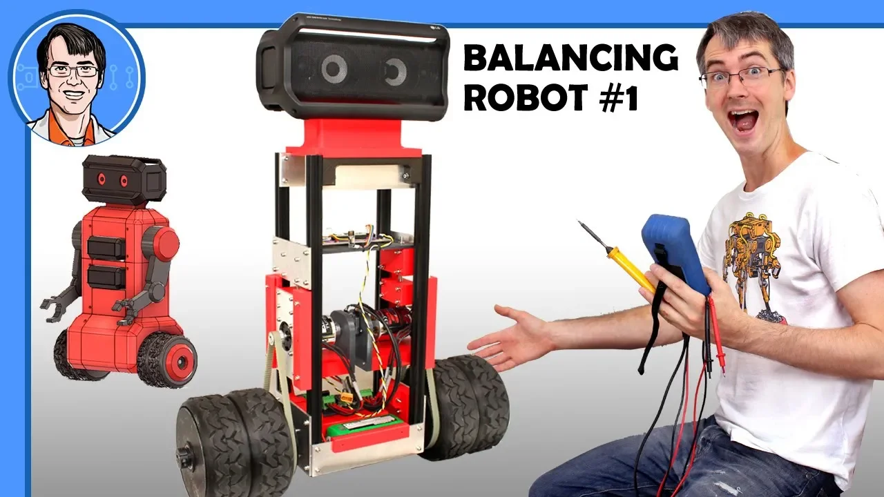
Why this video is valuable: This short video highlights how to set up the proportional and derivative feedback loops on a balancing robot. It provides physical intuition for how a robot reacts to tilt disturbances, which is crucial for verifying that your calculated LQR control forces are driving the motors in the correct direction.

---

Implementation Guide: Matrix Math on Teensy

Because running state-space equations on microcontrollers has limited video documentation, use the following guide to implement your C++ math:

You can use the popular BasicLinearAlgebra library (available in the Arduino Library Manager) to write clean matrix equations in C++.

#include <BasicLinearAlgebra.h> using namespace BLA;

// Define system state dimensions (e.g., 4 states, 1 control output per axis) // State vector: x = [position, velocity, angle, angular_velocity] BLA::Matrix<4, 1> state_vector; BLA::Matrix<1, 4> K_gain = { -1.5, -0.8, -12.5, -1.8 }; // Values computed in Python/MATLAB BLA::Matrix<1, 1> control_u;

void executeLQR() { // Read your filtered sensors and encoders to update the state vector state_vector(0, 0) = robot_position; state_vector(1, 0) = robot_velocity; state_vector(2, 0) = filtered_pitch; state_vector(3, 0) = raw_gyro_pitch_rate;

// Perform state feedback calculation: u = -K * x control_u = (K_gain * -1.0) * state_vector; float motor_effort = control_u(0, 0); // Scale and write motor_effort to motor driver PWM pins writeToMotors(motor_effort);

}

---

Step-by-Step 3D Ballbot LQR Tuning Methodology

Unlike a 2D cart-pole, tuning a 3D Ballbot requires a systematic, multi-stage approach to prevent damage to the mechanics:

1. Isolate the Axes: Suspend the Ballbot so the sphere rotates freely without touching the floor. Test individual motor directions to ensure a positive virtual control effort translates to motor rotation that physically counteracts the tilt.
2. Angle-Only Stabilization ($Q_{\theta}$): In your Python/MATLAB script, set the position states in $Q$ to zero. Set a high weight on the tilt angles ($Q_{\theta} \approx 100$ to $500$) and a moderate weight on control effort ($R \approx 1$). Compute $K$ and upload the gains to the Teensy. The robot should now actively resist being tipped over but will drift slowly across the floor.
3. Add Position Control ($Q_{pos}$): To stop the floor drift, slowly increase the position weight in $Q$ ($Q_{pos} \approx 1$ to $10$). Recompute $K$ and test. The robot should now balance and actively return to its starting coordinate when pushed.
4. Tune Angular Velocity ($Q_{\omega}$): If the robot oscillates rapidly (shakes) while balancing, increase the damping weight on angular velocity ($Q_{\omega}$). If it reacts too sluggishly, decrease $R$ to allow more control authority.

Knowledge Checkpoint

• Configure a hardware timer interrupt on the Teensy that executes a callback function at a deterministic $200\text{ Hz}$ frequency.
• Write a C++ function that multiplies a $1 \times 4$ gain matrix by a $4 \times 1$ state vector without using dynamic memory allocation (which can cause heap fragmentation).
• Implement the step-by-step LQR tuning sequence to safely stabilize your physical Ballbot on its sphere.
• Explain how you would modify your state-space matrices to add a yaw-rotation constraint, keeping the robot facing a fixed heading while balancing.

---

Course Map

This flowchart shows the recommended progression through the modules. Note that Module 2 (Kinematics and Modeling) and Module 3 (Sensor Processing) can be completed in parallel before merging into the control design and embedded implementation phases.

---

Key People Index

• James Bruton (Toymaker, Robotics Designer, ex-Toy Industry): Known for his open-source robotics projects (like HAL9000 and the openDog series). His practical videos bridge the gap between abstract physics equations and physical 3D-printed hardware.
• Prof. Steve Brunton (University of Washington): Creator of the popular Control Bootcamp series. He provides exceptionally clear lectures on dynamical systems, state-space representations, and optimal control theory.
• Prof. Christopher Lum (University of Washington): An expert in aeronautics, flight controls, and systems engineering. His deep-dive lectures on LQR offer rigorous, step-by-step derivations of the algebraic Riccati equation.

---

Final Self-Assessment

Test your understanding of the complete Ballbot design. You are ready to build the physical robot when you can check off every item below:

• Teensy Interface: You can read encoder pulses at $200\text{ Hz}$ with zero missed ticks and write direction-correct PWM signals to three separate motor drivers.
• Kinematic Mapping: You can transform desired directional movements in the $X$-$Y$ plane into the corresponding angular velocities for three symmetrically arranged omniwheels.
• Physical Dynamics: You can write out the kinetic and potential energy equations of the system and state how changes in mass distribution affect the system's natural frequency.
• State Estimation: Your Kalman filter outputs pitch and roll angles that remain stable under vibration and do not drift when the robot is at rest.
• State-Space Modeling: You can define the matrices $A, B, C, D$ for your physical robot platform.
• LQR Optimization: You can compute an optimal feedback matrix $K$ using python/MATLAB and explain how the weights in $Q$ and $R$ affect the poles of the closed-loop system.
• Embedded Execution: Your Teensy executes the entire state estimation, kinematics, and $u = -Kx$ matrix calculations in under $1.5\text{ ms}$, leaving headroom in your $5.0\text{ ms}$ control loop.
• Physical Tuning: You can successfully balance the robot on its sphere, observe physical oscillations, and adjust the corresponding LQR weights to damp out unstable behavior.