






![Espacio de Estados ► VARIABLES DE ESTADO 🤓 [Sistemas de CONTROL] #003](https://i.ytimg.com/vi_webp/BnCS3l3M09U/maxresdefault.webp)





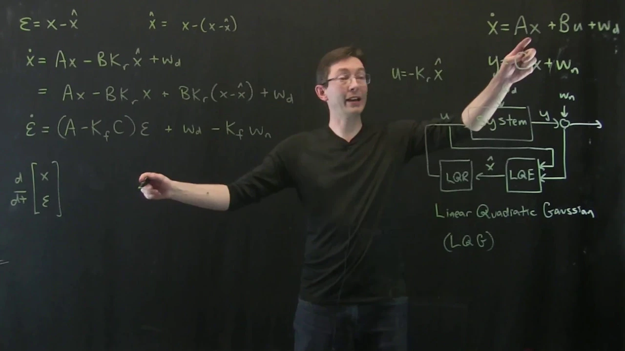






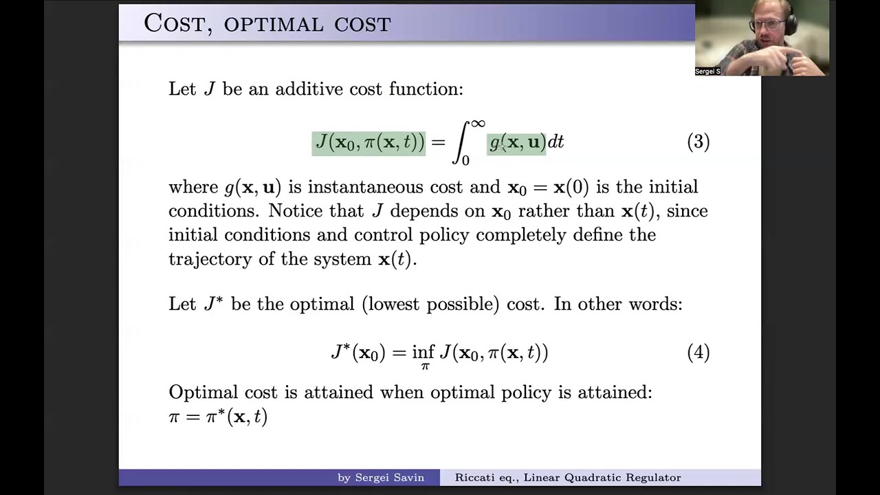




The Linear Quadratic Regulator (LQR) is a powerful control design technique that computes the optimal full-state feedback gain matrix K by solving an optimization problem, where the controller minimizes the cost function J = ∫₀^∞ (xᵀQx + uᵀRu) dt subject to the system dynamics ẋ = Ax + Bu; the matrices Q (symmetric positive semi-definite) and R (symmetric positive definite) serve as tuning parameters that allow engineers to trade-off between state regulation and control effort, with the optimal controller given by u = -Kx where K = R⁻¹BᵀS and S satisfies the Algebraic Riccati Equation AᵀS + SA - SBR⁻¹BᵀS + Q = 0.
Linear Quadratic Regulator (LQR) Control Design Tutorial
Added:State-space representation of dynamical systems, including state equations, input vectors, and output equations.
Fundamentals of state feedback control design and the concept of pole placement.
System controllability and observability to ensure the physical viability of feedback control.
Basic linear algebra, particularly quadratic forms, eigenvalues, and positive (semi-)definite matrices.
Linear Quadratic Gaussian (LQG) control, which combines LQR with a Kalman Filter for systems with noise and unmeasurable states.
Solving the Continuous and Discrete Algebraic Riccati Equations (ARE) both analytically and numerically.
Model Predictive Control (MPC) to extend LQR concepts to systems with strict state and control input constraints.
Robust control theories, such as H-infinity control, to handle model parameter uncertainties and external disturbances.
148.5K views3.2Klikes1:36:06Original Release: 2018-12-03
hello everyone and welcome to another video today I'd like to talk about one of the most popular and powerful control design techniques around the linear quadratic regulator or lqr controller we're gonna see that an lqr controller is effectively a full state feedback controller where the gain matrix K is computed in a very particular fashion I'm gonna assume that you're a little bit familiar with full state feedback control but if you'd like a quick refresher please check out this previous video where we introduce full state feedback controllers we're also gonna see today that lqr controllers address some of the practical implementation issues we encountered when designing full state feedback controllers so to get the most out of the discussion today I recommend that you also check out this other previous video where we discuss some of these implementation problems links to both of those videos are in the description below so if all of this sounds like more fun than a clown on fire let's jump over to the whiteboard and get started all right so let's talk a little bit about the linear quadratic regulator or lqr controller right so like we said earlier the deal with an lqr controller is that let's assume that we've got a plant here it's a linear plant of our standard form here but the output like we said earlier is the entire state of the system so if you have this scenario we said last time that pretty much the most powerful controller you can use here is a full state feedback controller like this right so here's your full state feedback controller right and the whole game plan at this point was to just to choose K so last time I think we showed here that you can basically try to tailor how the full state feedback controller behaves by choosing desired closed-loop poles of that entire system right I think last time we said that you know if you had some some plant here with with certain open-loop poles here right by the represented by these blue X's here right so these blue ones are open-loop poles in other words it was basically eigenvalues of just the a matrix right and what we said later was that okay I can just go over to MATLAB and I could say place a B and some P desired right and this would give me a matrix K or it will give me the controller that would move the open-loop eigen values in other words these blue X's to wherever I desire it to go here right where is this this P desired so we saw that by choosing locations of say say I want to move them you know something like this here right where these green ones are now my desired poles these are my pedas iured we saw that by changing these locations moving them further or closer or moving only certain poles right we could somehow mess with what value K was but this was a little bit unsatisfying in the sense that there wasn't a real knob or a way to twist and and physically understand how the changes of these Green X's affect the controller or affect the behavior of this overall system here right so that was the problem with full state feedback controller it was that it was a little bit difficult to understand the relationship between P desired and the resulting K well this is exactly the problem that lqr is gonna allow us to address here what we're gonna do here is try to pose this entire problem here in an optimization framework so optimization is is one of the most powerful branches of mathematics in fact I've heard a couple people say that you know it's it's it's probably the most important engineering topic here that that almost any problem in engineering can be posed as an optimization problem if you think about it long enough here so what we should maybe do here is let's take a brief sidestep and talk a little bit about what is optimization and how can we maybe apply it to this scenario so to set the stage for the concept of optimization let's talk about my daily commute for those who don't know me I live in the Pacific Northwest specifically I live on Bainbridge Island which is about 10 miles west of Seattle Washington and I work at the University of Washington which is actually on the other side of this large body of water called Puget Sound so the problem I'd like to consider now how can I commute from my house to my work every single day why don't we brainstorm some possible solutions to this problem now luckily for me the state of Washington operates the largest ferry system in the United States so one option is I can just drive from my house down to the ferry terminal put my car on a ferry mode go across the sound and when I get to Seattle just drive the rest of the way up to the University of Washington so let's call this solution maybe z1 where I Drive from my house of the ferry catch the ferry and then drive to campus what else could we do well if I don't want to drive maybe I'll catch a bus from my house the ferry terminal walk onto the ferry mode and then when I get to Seattle just buy some bus that happens to be going to the u-dub so here that's z2 here bus ferry bus what about a third solution well if I want to get some exercise why don't I ride my bicycle to the ferry terminal and then I can actually put my mic on the boat take it across the water and then when I get to Seattle ride the rest of the way up to the University of Washington great so z3 bike ferry bike why don't we think outside the box a little bit I could maybe now run from my house to the nearest shore line of Bainbridge Island hop in the water and swim five miles across the sound here and then Forrest Gump it to campus and arrive more tired than that creepy dwarf and Snow White but you know what z4 where I run swim run is is actually a feasible solution all right let's just skip all to this hoo-ha and I'm just gonna charter a helicopter to take me directly from my house and drop me off at my desk at the University of Washington every day so z5 is just charter a helicopter you know what this sounds good so why don't we stop here let's call this entire set of all possible solutions the feasible set the feasible set is basically every solution you would like to consider when solving an optimization problem okay so we saw that we had all of these potential solutions and we said we're going to call a collection or a set of all of these maybe Big Z and we'll just put all of these solutions in here and this is what's referred to as the feasible set so now that we have the feasible set put together the next thing we need is we need some way to measure the goodness of each one of these items in the feasible set this is what's known as a concept of a cost function so the idea with the cost function is that it is literally a function where you pass it in an element of the feasible set so it's one of these Z's here and all this thing's job is it's got one job right is it needs to evaluate how much does that item cost here okay so what will come out of this is let's call this cos J of Z here right so again this is typically we're going to use a notation J here so J of Z is going to be the cost function that measures how much solution Z costs right so this could be in terms of dollars or any other abstract metric as long as it's a scalar value here right where you pass it in an action and in action you know it could be something complicated like all of these or it could be a vector it could be some item right at some solution this thing gives you the number of dollars here ready to gives you a single value which measures that right so what we're gonna see here is that the optimization problem involves finding a feasible solution here that will minimize the cost of a given problem here right so tell you what let's consider a bunch of different cases here so let me erase some of this we can get a little bit of space so I'd like to consider a few different scenarios here so let's look at maybe case or scenario 1 here where I want to minimize time okay so in this case what I'd like to do is I'm going to develop a cost function let's call it J 1 of Z here right where what this cost function does is it just measures the time required for action Z right so in this context of the problem here or the optimization let's write it here as maybe p1 here right is I want to minimize j1 subject to the constraint here that I'm not going to consider all possible solutions I only want to consider the solutions here that are in my feasible set here right only these five that we laid out here right so if you look at this what the optimization problem says is I need to find the element in the feasible set which basically will yield the minimum time for my commute here right so if you look at this here right we get we can iteratively by brute force just go through every single one of these and evaluate how long they each take um and and the winner is going to be z5 here right you can pretty much see that out right off the bat that this is gonna get me from my house to campus in the minimal amount of time here so in this scenario here right the thing that is optimal here is z5 is optimal right okay well um how about let's consider another case how about case two maybe let's underline these so we can keep them apart case two here how about how about let's minimize money right so instead of time being important let's say I'm super cheap and frugal and I care about money so I need to develop a second cost function J 2 of Z this cost function the only job in life here is to measure literally the cost of action Z right so how many dollars does each one of these things cost so I can form an entirely new optimization problem let's call it P 2 right where I now same thing I want to minimize this other cost function J 2 here again I'm only gonna look at solutions in my feasible set here right so I go through each one of these and I ask how much does this cost here well it cost me some gas and then to catch the ferry I actually have to pay to take my car across that cost me some gas again oh here Z 2 this is actually a little cheaper here because I don't have to pay to take my car across the ferry I could just walk on which is actually much cheaper oh this is easy this is also kind of cheap here but oh hey check this out z 4 this doesn't cost me a dime here right nobody I can run for free to the shoreline it doesn't cost me anything to swim across what it doesn't cost me any money maybe a let's put it that way it might cost me other things but doesn't cost me any money to get across Puget Sound and I could run and whoo crud dzifa okay the helicopter is definitely gonna cost me a boatload of cash here so you know what in this scenario here with this cost function the optimal thing does it do is actually Z 4 right huh so this is really interesting here in the sense that this same optimization problem we can change the solution by picking the cost function appropriately so tell you what let's go ahead and look let's make another variation on this how about case three here let's try to look at a minimizing a time and money trade-off okay so in this case why don't I make a cost function let's call it J 3 which is actually a combination of these two here so let's have J 1 here remember J 1 returned the time required and I'm going to add that to J 2 which measured the cost here and what I could do here is I could put some scalar weights in front of these here which would allow me to sort of trade-off between how much do I value time versus how much do I value money here right so in this case Q and R are scalar let's call them weights right that we can use to tune the optimization problem here right so you know if you look at this you can basically see here that depending on on Q or R you can say do I care more about time or do I care more about money so just to kind of write this down right if you look at this here well again maybe we should write down the problem here right so the problem is the same thing so P 3 is now I just want to minimize this new cost function J 3 of Z such that subject to Z is in our feasible set big Z okay so depending on what values of Q and R we choose you probably get different values here right so in general right you can see here that a large Q relative to our right what is that going to do here right that's basically saying that you're reverting to a minimum time problem right because if Q is big then if the time is big this be that the co entire cost function becomes big here so you really want to choose solutions that minimize time here so if you do this here this is basically saying you also made relative to our right you're you're super rich and your time is more important than your money here right so if you do this you say what we're basically doing here is this this this kind of revert to a min time problem right basically revert Stu this case here right so we see that all right in this case you end up again back with with our z5 solution of just getting the helicopter right alternatively if you have a small Q relative to our right this is now saying that no actually you're super frugal right you don't have any money so any expenditure of cash is is very very bad here right so that means that our sorry where was I put ya R is larger than Q here right so what this does is what this revert to a minimum money problem here right so here this solution comes back to being Z 4 here right which makes sense now where it gets really interesting here is what if you have a trade-off between Q and R right in this case this is a new scenario right where now it depends it depends how much do you value time versus how much do you value money so in this case we have what we have potential solutions I don't know which one is going to be optimal again it depends on what values of R but now you've got a Z 1 Z 2 or maybe Z 3 as being reasonable solutions here all right let's explore this a little bit further here let's think of maybe a case of 4 so let's do this right here unfortunately didn't manage the board space extremely well here but let's look at case for case 4 is basically I'd like to look at case 3 again right this interesting where we're trading off time and money but I'd like to add what are called constraints okay so what constraints allow us to do here is further tailor the solution to this problem here by eliminating values in the feasible set so what this does here is again let's restate our problem here so I'm gonna I'm gonna call this P for now here but again it's it's the same cost function as case 3 right so I want to minimize J 3 right this was our trade off cost function here subject to elements in the feasible set here and I'm gonna tack on some additional constraints here as something like what if I say I want to make some kind of requirement here that I need to get 30 minutes of exercise during my commute or more here so what I'm gonna do is I'm gonna make up a function let's call it f1 here right where f1 job here is that you put in one an element out of your of your feasible set here and what this measures here is it measures the exercise time associated with action 0 right so the optimization problem becomes what we saw earlier but as well I'm gonna specify a constraint like I need F 1 of Z to be greater than or equal to 30 minutes here so this is basically saying that on my commute I also want to make sure that I get 30 minutes of exercise what this does by specifying this additional constraint here is we see that it starts making some of these elements in this original feasible set infeasible so for example if we look at all of these here let's let's just walk down these one at a time right how much exercise am I going to get out of each one of these so z1 here right z1 if I pass this through my F function it's gonna look and say hey you spent 0 minutes exercising because you're just walking in or driving in the car then you sit on your bum on the ferry doing nothing and then you drive some more so this actually does like nothing so this is now not going to be allowed any longer here so z1 is no longer a feasible solution same thing with z2 you're just sitting on the bus and sitting on the ferry so f1 this function here or this constraint that we cooked up is going to say no that's not allowed any longer okay z3 this is a yeah actually this is still allowed because you're gonna get a lot of exercise biking here on either end so this is allowed oh man z4 is definitely allowed right you're probably gonna get more exercise than you want here and then the helicopter becomes infeasible because you don't get any exercise on this helicopter here right so suddenly this problem here now it gets a little bit simpler because the feasible set shrunk so there's only two solutions here you can either bike or or run and swim here right and usually for most values of R and Q and R right you're gonna see that that Z for solution that's going to take that's gonna take hours and hours and hours and hours so usually this this term here the the the the cost function that's measuring time is going to make that Z for solution really unattractive so in this case here what's probably going to happen here is we're gonna end up with Z 3 is optimal right so this is really fascinating in a sense that depending on how you tailor your optimization problem right the solutions change here what is considered optimal changes here right so this is actually really interesting and now the question would be how can we apply this optimization framework to designing a control system for a linear dynamic system so let me erase the board and we'll jump into that next ok now that we've got that basic understanding of general optimization let's think about how we can set up the optimization problem for designing a linear quadratic regulator here so let's talk real quick about setting up the optimization problem so I always think it's easiest to think about a concrete scenario so you know what if we had something like like like a satellite here so I'm gonna try to draw a satellite here I'm obviously not a very good artist I think those of you who have seen some of my other videos understand that but I'll just make some little cartoon here for a satellite here and what we'd like to think about here is this satellite might have multiple states here right so the state vector for this satellite might be something like the orientation right there might be states for the for the Euler angles there might be States for like the position all these other things right we will just stack all these up in the state vector and at the same time this aircrew this satellite might have multiple different controls right it might have like a primary thruster here it might have smaller positioning thrusters or or momentum wheels or things like that here so we might want to also say that this thing has multiple controls here right so this would be like the like the main thruster you know electric thrusters momentum wheels etc etc etc right well all we're getting at is that this here is a dynamic system which has multiple states and multiple controls simultaneously let's go ahead and assume that this is a linear system governed by dynamics of X dot is equal to ax plus bu right our normal state space representation of my dynamic system basically saying that the state and the control they're not free to be anything they want right there's a relationship between how the states and the controls interact and they interact through this dynamic equation here right so within this context here what we want to do here is let's set up an optimization problem here so the optimization problem here is let's go ahead and consider a cost function let's just call this thing J like we did earlier here and we're gonna propose this cost function here it's going to be the integral from x 0 to infinity of x transpose times some matrix QX + u transpose some matrix R u DT okay so here's our cost function here in this case we see that XR obviously is your n by one state vector right U is our usual M by one control vector and here Q is a n by n symmetric positive semi-definite and we'll talk about the definition of that here matrix here sometimes you'll see this written as q greater than zero or sometimes you might see q like this kind of script e greater than zero here again this is a notation for this matrix is positive yes positive semi definite here and finally R is a M by M symmetric positive definite matrix again sometimes written as q oh wait mom I'm sorry sorry okay come back to the sorry come back to the Q here positive semi definite means greater than or equal to sometimes it's written like this to contrast it with positive definite which means that it well what we'll get to that in a second again you might see this written as something strictly greater than or again this this script e greater than symbol here right okay um maybe now might be a good idea to discuss what is the definition of positive definite and positive semi definite let's come back to this and I'll let's delete our picture here I think we understand the scenario that I like to keep in the back your head so just keep and keep in your head that you know the state vector here let's let's think about this as being a state vector for the satellite and the control vector being as a control vector for this particular satellite here so the the concept here with a positive semi-definite here so maybe a let's write that down so positive semi definite means that this matrix Q if you took it and multiplied it by some vector X transpose and then multiplied it again by this is a skate going to be a scalar number here if you if you do the dimensions here right this is n by one by an multiplied by an N by n multiplied by an N by one and excuse me invited time you transpose this thing this becomes 1 by n right so you can see the whole thing ends up as a 1 by 1 scalar here right this scalar quantity is always greater than or equal to 0 for all possible X values here right so that's the definition of positive semi-definite is that this matrix is positive semi-definite if when you compute this weird quantity X transpose QX it is stricted it's greater than or equal to 0 for any value of x this vector right this this vector could have positive negative zeros whatever it doesn't matter by the time you run it through and compute this you get something that is strick is greater than or equal to 0 all the time here right similarly the definition of positive definite right is that again you have this this this this matrix R here which we claim is positive definite the definition is that if you take some vector you may be in this case transpose times u this is strictly greater than 0 for all u right so again you can work out the dimensions that you see that this is a scalar number here so here's the definition of positive semi definite and positive definite and what's interesting about that is that is exactly what are the terms of the integrand of the cost function here right so you see that the reason the way that this cost function is set up here is that the integrand is always positive or or as well actually yeah it's it's positive right for any X u combinations here right so you can never get a negative integrand the integrand is always positive so let's let's keep that in the back of our head as we continue discussing this ok all right so now that we understand positive definite and positive semi definite we have a we have a rough kind of feeling for what this this cost function does right you can kind of see here that again the integrand is always positive and q and this are those are sort of these waving matrices or weighting values that we saw earlier when we were looking at our brief introduction to optimization right we earlier the Q and the r were somehow to trade-off between time versus money here right in this case we see that Q and R trade-off between states here non zero states or non zero controls we're gonna take a closer look at that in a second but I wanted to plant that seed in your head right now let's start thinking about Q and R as weights to get to determine how much we value States versus how much we value controls here right okay so now that we have the the cost function down the overall problem now in this scenario here is actually table maybe let's let's do it over here so we can keep talking about that the problem here so here's the cost function so the optimization problem let's write this again as our script DP symbol here right is all I want to do now here is I want to minimize this cost function J here right but the controls I want to use here right there's M controls here so U is is a real valued M valued vector here right but we're not it this is not unconstrained here there's a certain constraint right such that the single constraint that we want to consider here is that again xn you are not free to be anything you want here right it's X dot is equal to ax plus bu right so here is my optimization problem that I would like to solve here right and if we think about this long enough what it's basically saying here is that you want to take this cost function here and I want to find some control signal or some control law that is going to make this cost function minimal the so first of all let's stop it let's think about that first look for ignoring strain turn ow right how would you make this minimal here so for example assume that your satellite had some nonzero initial candy like X of 0 was not equal to 0 in other words your satellite was cocked over at some weird orientation and some weird position not 0 all right it's something that you that you didn't want here right so this term is non 0 at time 0 right now if the satellite stayed there right if you left it here like let's draw a quick picture maybe of just one of the states like X 1 right if it's here's our initial condition right so so maybe it is banked over at 45 degrees away from where you wanted to write if you left it here right it did nothing right what does this cost function look like here you can kind of see it already it's getting there there's gonna be a square there's give me an X 1 square term here multiplied by this Q let's assume that Q is like all ones or something like that effectively what the cost function there is measuring it's it's sort of measuring the integral of this right of course it's gonna be squared it might be skewed or weighted by that Q value we're gonna see that in a second but long story short here if this stayed here at a constant value this cost function is going to blow up to infinity here right because it's it's the integral from x 0 to infinity here right so you can't have this here right this is obviously not the optimal thing to do here you can't leave this satellite cocked over at 45 degrees because that yields a cost function value of infinity here right so that's obviously not a good thing to do so instead what is better here right is we should try to bring the system back to the origin here right and now the cost here is finite right it's just sort of this area under the curve is the cost value so this is a better solution than letting it stay at 45 degrees so what that means is your satellite is cocked over 45 degrees what we're gonna do here is is maybe bring it back to 0 that yields a better result here right however the other flip side of that story here is how are you going to bring the satellite back to zero here well you're probably going to have to fire some thrusters right some positioning thrusters you're going to have to expend some amount of trol in order to do that here right so if we plot again this is a real rough shooting from the hip description of this we're gonna look at it in a more formal fashion in the second here but let's just plot one of these controls like maybe U of T this is like one of the positioning thrusters or something like that right well what you're gonna probably have to do is is if you want to bring the satellite back to zero you're probably gonna have to expend some control authority to do that and then again you're probably gonna have to let this come back to zero here right so you're going to actuate the controller and like you're gonna bring it back to zero then you're gonna stop actuated the controller right so the overall cost function you can kind of see it's sort of a combination of both how long are you away from zero in the States and how much nonzero control authority did you actually have to expend in order to get that here right so what you can see from this discussion here is what Q and R do are q and r are these knobs that allow you to determine how much do you care about the state being zero versus how much do you care about the control not being zero here so let's talk about that real quick in general right what you end up seeing here is that you know roughly speaking if Q is is big compared to R so maybe we should write that down here right so if Q is bigger let's put this in quotes here then our the reason it's in quotes here is because if you can call you can see Q and R they're two matrices they're square they're symmetric but they're not even like the same size so how do you really say one is bigger than the other here well we're gonna get to that in a little bit but you can kind of you can see the gist here right if Q is bigger than R here what are you basically saying you're basically saying here that I really care that X is not equal to zero because if so this this term dominates here right so in this situation let me do is in another color here right this term dominates so really all you're seeing here is the important thing this case here is that if the states are not equal to zero you end up with a huge cost here right who cares about what the control is it's really the states that matter and drive this cost function here so in this scenario what do we end up with this is basically saying here the optimal thing to do here is do what you have to button make sure those states go back to zero as soon as possible here right so this is typically going to yield something like you would have a fast regulation of X to zero right and in order to do that you're going to end up with u is large right so this is sort of the scenario where you're saying control is cheap I don't care what you do just make sure the state goes back to zero really really quickly here right let's flip that and and and compare with you know what happens if R is bigger than Q right so in that case we have the exact opposite scenario here right where now it's this term that dominates in the cost function right so the optimal thing to do here is make sure that you stays as small as possible here because if you even flinches up four or flares up if you actuate one control just a teeny a little bit this term and your cost function is going to blow up and you're going to end up with a huge cost here right so the entender this situation the right thing to do here is use control very very very sparingly here right and who cares what the state ends up doing in this scenario if it stays if the satellite stays cocked over and just takes you know hundreds of seconds to come back to to the origin that's fine as long as you don't fire those thrusters because the propellant you're expending is is extremely valuable here right so the behavior that typically ends up happening here is you know if you have are bigger than Q here you have very slow regulation of next to the origin here right and you is small right so this is really interesting here so you end up with it is the the first case here this is like an aggressive controller right and down here you have a bit of controller so we see that Q and R these knobs that are going to allow us to to tweak the states and the controls or excuse me tweak the controller depending on how much we care about the states and controls let's look at a very concrete example the collection I think we'll be able to see that here so for example here right let's look at a two state to control system right so what if your satellite here that we're looking at it only had two states like like we were looking at just the sorry let me just write this down so I can I can talk at the same time here right there's only two states like maybe I only care about the pitch angle and the pitch rate or something like that of it and then I only have two controls here like I have a electric thruster and a single momentum wheel or something like that right okay and now let's let's pick values of this Q and these are matrices here so in other words let's first start with something really really simple let's make the Q matrix just diagonal and I will have a q1 one and a q1 it sorry q2 - let's make zeros over here similarly for the r matrix right r is just going to be an r 1 1 0 0 r 2 2 right ok so these are these are these are symmetric and as long as all of these these entries are positive we'll see that these yield a positive semi-definite and a positive definite matrix here right so if this is the case let's compute this cost function here or more importantly maybe let's just compute the integrand of the cost function here maybe let's see what can we do yeah yeah let's listen so I think we got they got the picture here ok so now what I want to do here is are its compute the integrand here right of X transpose Q X plus u transpose or you right--so run to Mathematica and plug all this in here and what you'll end up seeing here is that this integrand looks like it's it's pretty simple it's a q 1 1 X 1 squared well has a Q 2 2 X 2 squared it was with a squared like this sorry plus an R 1 1 u 1 squared plus an R 2 2 u 2 squared here right so here I think you can very clearly explicitly see what do these q 1 1 and Q 2 and 2 2 and R 1 1 and R 2 two entries physically mean right if you look at this right we see that what Q 1 1 is sort of the the weight or the the penalty effectively on a non zero X 1 right because it shows up right here right so if X 1 is not 0 right um if it's positive or negative by the time you square it this term is going to be positive here right so as long as the magnitude is not 0 this squared term is something positive and Q 1 1 is now this this multiplicative factor here is showing you how much does it matter that X 1 is not 0 here right it will either exacerbate that in terms of the cost or would attenuate it depending on on this value here right and similarly let's just go through all of these just to be very very explicit so Q 2 2 right this is the weight or the penalty on a non 0 X 2 right so we very clearly see that the Q matrix by choosing the entries appropriately you can now say which state do I really care about being nonzero right I can either say that I really care about x1 being nonzero or I care about x2 being not 0 similarly the r11 term right you see it right here right this is the weight or the penalty on a non 0 u 1 of T right and similarly R 2 2 is just the weight or the penalty on a non 0 u 2 of T right so R 1 1 is basically it's it's actually telling you pretty much exactly how expensive is it to fire or to utilize control number one all right this was like maybe your electric thruster maybe it doesn't cost you anything at all right because that's the whole deal of the electric thrusters is that electric thrusters are are cheap they're long-lasting they're reliable here so so if you want to model that fact here in your control design you can maybe pick up pick a small r11 right because if r11 is small it's basically saying I don't care what you're doing with this controller this controller is SuperDuper cheap because even though if this control is is is large by the time I multiply by a small r11 this doesn't contribute to the overall cost function much right and in the same fashion you see that r22 is is the is the cost of actuated controller number two here right so that's pretty awesome this I think allows us to set up the entire optimization problem here right now the thing that's interesting here is now if we start coming back and thinking about the the constraint here right this is the interesting part we I think we understand the cost function at this point right and we understand how to tailor or to tune this cost function using this Q and this R matrix here right but the thing that we have to do now is we have to solve this overall problem now here subject to the linear dynamics of this system here right so that's where it gets interesting so why don't I pause the video I'll erase the board and now let's talk about after we set up the optimization problem how can we solve this optimization problem okay so now what we'd like to do here is look at solving the optimization problem so graphically what this means here is again here we've got our linear plant right which is governed by X dot is equal to ax plus bu right and now what I want to do is I want to find a control law u here which is going to make this whole system here optimal here right so I'm going to use au here so that the X by the time I look at the combination of U and X and that cost function it stays small according to the cost function that we set up here right so it turns out that the solution to our problem here so I'll just write this down here so the solution to our optimization problem here right which was we said earlier minimize this cost function of integral 0 to infinity of X transpose QX plus u transpose ru DT subject to these dynamics here right this was the optimization problem here well some really smart people figured it out it's beyond the scope of this lecture today to derive it here but I think we can use their result here the solution here is that you better choose a control here that looks like this - KX of T where this game K here is given by R inverse B transpose s here and s is the solution to what's called the algebraic riccati equation of this so a transpose s plus si minus SB r inverse or the R inverse B transpose s plus Q equals 0 here right ok great um and here ya s is a solution algebraic riccati equation and also it is its size n by n + square and symmetric ok so this is the solution here right so tell you what if we first if we first ignore everything below here just look at you look at the solution here right solution is minus KX we've seen that before this is just a full state feedback controller right so in other words the arc texture that goes along with this is that this thing just looks like minus K right so the optimal thing to do the absolute best thing you can do to solve this problem is to use a full state feedback controller here now what gets interesting here is that the way you get this K here you have to go through a couple of steps here right if you look at this so step one here is we got to solve the algebraic riccati equation for s here so let's talk about this the so the procedure for lqr right so step one here right we are going to be given our a and B matrix right those come from the plan right those are known right okay they're known and immutable you can't really change them the next thing we have to do here is you you are gonna pick the Q in the are right because you as a control designer you get to choose how much do I care about states versus how much do I care about control actuation here right so you choose that the cost function effectively here right so let's say step two is choose Q and R right you're basically designing the cost function now according to this step 3 here's once I have Q and R I need to solve the algebraic riccati equation for s here right so solve I'm just gonna abbreviate this as a re here right so this down here is the algebraic riccati equation here right okay so you solve the algebraic riccati equation for s alright what you're gonna end up seeing here is that once you solve for s there's actually going to be multiple solutions to s we'll take a look at this in a second here but if you follow a couple of steps you'll be able to find out which is the one you want here once you know that here well actually no I take that back let's just say solve this thing for s you're gonna get multiple solutions therefore you can then compute K you're gonna get multiple solutions for K here right so you can go ahead and compute your optimal gain K using our expression over there right R inverse B transfer Transpo's s here right and again since there are multiple solutions of s you'll get multiple solutions for K here the last thing that you have to do then is typically there's only going to be one solution here that yields a stable situation here so if you remember earlier with this control of a full state feedback here right this thing is basically going to behave at the end of the day like X dot is equal to a minus BK X right and this here is like maybe your your a closed loop a matrix here right again if if this is if this is brand-new to you here maybe take a quick refresher here to our video where we discussed full state feedback controllers but we showed that under this control law the dynamics reduced to this here right now what you can do here is you've got multiple k's here right so that means you have multiple A's closed loops you can evaluate each of these eight closed loops and find its eigenvalues and usually there's only one of them that are going to have all poles in the or eigenvalues in the left half plane here so let me let's say step five here is choose the k's solution that yields a stable system yeah so that's the workflow that we need to go through so again I love concrete examples let's look at a concrete example right now to try to implement all this so the example I'd like to use here is a really simplified scenario it's a a mass and a damper that's it okay so let's look at an example here of a mass / damper system so you've got some smooth surface like I don't know like some ice or something like that you got a mass sitting on this thing and all we're gonna be doing here is let's consider the position and the velocity here like such positive position and positive velocity as to the right here and let's say that you have a single control of this you're able to exert some kind of force on this block so you maybe have one rocket engine or one thruster that pushes this block along this ice here and here there's some viscous damping between the block and the the surface here alright so I think you can get without too much of a stretch of an imagination here that Newton's second law equations of motions are going to give a to give you mass times velocity acceleration right is equal to the sum of all of the forces here right so you got the force here minus the retarding force of the ice here right P times a C or sorry C times P dot here right okay so without too much um oh sorry I said we should say viscous damping with coefficient C all right that's what this C is here it's just how much friction you got okay so without too much of a stretch I think you can turn this thing into a state space representation here by choosing a state vector X of T as let's make it the position and the velocity of the block that's our state vector and the control vector in this case is actually really really simple there's only one control it's this force right okay if you do this here you can basically get yourself a a state space representation of X dot of T is equal to 0 1 0 minus C over M X plus 0 1 over m you great that's our state space representation here's our a matrix here's our B matrix here let's go ahead and choose some numerical values so we can actually try to compute some of these here so let's go ahead and how about consider a mass of 1 and us coefficient of damp damping here of 0.2 so numerically we end up with an a matrix that looks like zero one zero minus one-fifth here and a b matrix that looks like zero one okay something pretty simple now that is that step one here right we got a and B okay step two here is let's choose Q and R okay so I don't know let's pick this like a Q just something really simple how about an identity matrix here later on we're gonna look at some examples where they're not identities but okay q is identity matrix R I don't know let's choose something like 0.01 something like that okay great so we got step 1 and step 2 now done now we got to go ahead and solve ourselves the algebraic riccati equation here so that's a little bit of a pain in the neck here right because if you remember that's this long matrix equation we got to set it equal to 0 and solve for s here so I don't want to do that on the board let's do actually steps through five here let's just run over to Mathematica and have it do this for us so we can see how can we compute this game K all right so I'm gonna pause the video and I'll meet you over on Mathematica alright so here we are in Mathematica so why don't we go ahead and make a couple of notes here so what we would like to do now is demonstrate solving the AR the algebraic riccati equation and computing and lqr controller okay right that's our game plan here so we said her let's first do step one right step one was define the a and B matrix right so I think what we said was a was just a very simple what was it 0 1 0 minus 1/5 I think and then B was pretty simple 0 & 1 okay there we go shift enter that guy and here's step 1 uh what was step two step 2 was go ahead and choose Q and R right so I think in our situation we said that the Q was just going to be a very simple identity matrix here and the R matrix is actually going to be a 1 by 1 of 1 over 100 here so let me just define it here as a list of lists here it's just that Mathematica as well it has a little bit of trouble using the parenthesis notation to make a 1 by 1 matrix here so I'm gonna just explicitly make a 1 by 1 matrix here okay shift enter both those okay now we're on to step 3 we said which was solve the a re-write so just to refresh your memory here right the the Debray riccati equation is given by what are we saying was I think it was a transpose s plus si minus SB whoops R inverse B transpose s plus Q equals zero right so we want to solve this for s here right okay so let's just go ahead and compute the left hand side of that expression first so the left hand side here is what it's just transpose a times s plus s times a minus s times B times inverse of our times transpose of B times s plus Q right so that's the left hand side here and maybe let's just simplify maybe let's put the simplify up here whoops did I spell that wrong simplify here right and then let's just look at this thing in a matrix form just to get an idea of this so wait a second oh I'm sorry here we should have defined s here right so um we know here that s is what it's a symmetric matrix here so there's going to be an s11 and s12 and this is also going to be an s12 because it's symmetric and then have an S 2 2 so this is what s looks like here so maybe let's make a quick note of that here and Mathematica notebook here so define as a symmetric matrix of size n by n right ok now this second step here is go ahead and solve the a re ok so let's see shift enter this value of s here's shift enter the right hand side here we go so here's what it looks like right so we see now we basically have again this is actually a symmetric equation here right our symmetric matrix if you look this off diagonal entry is the exact same as this off diagonal entry here so really we have three equations and three unknowns right I need to find s11 s12 and s22 here right so what I need to really do now is I need to say solve basically the a bunch of equations right if the left the one one element right this has got to equal zero actually all of these entries have to equal zero so this s equals zero the left-hand side of one two has got also equals zero and the left-hand side two two has got to equal zero right so those are the this equation has got equal zero this has to equal zero and this has to equal zero here right those all solve them simultaneously for what s11 s12 and s22 right that's what I'm looking for here right so if I shift enter this you see that we actually have four solutions like we said earlier right that was to be expected we said that when you solve this for a lot of times they're going to be multiple solutions for s so let's just go ahead and extract those here so maybe let's assign this to a temporary variable call it temp and um let's see here s let me think about this how do we want to do this here you know actually we're ready to find s up here I know what we'll do let's just do it like this here so let's call this thing how about solution one gets temp one so this is the first set of solutions here all right let's do this for actually all four of them here right so let's get all four solutions here so let me see changes to a four three two and then solution two three four okay so here's our four solutions and what I want to do now here is make the four matrices here so s1 is going to get s but I want to make all of these appropriate substitution so I'll just say slash dot with solution 1 all right so here's s1 and great let's again do this for all 4 4 3 4 3 2 and then this should be 2 3 4 here and tell you what let's just go ahead and suppress the output for all these and then we will just look at these things as numerical values in matrix form just we can get a rough idea of what they look like oh sorry that should be s1 s2 s3 and s4 so we shift into those so we see here are the four solutions here to the algebraic riccati equation so we need to now identify which one these are the correct ones so let's move on to step four here step four which was compute K alright and if you remember here we said that the way we compute K here was K um sorry excuse me K is going to be what it's our inverse B transpose times s here so we end up with four solutions here so let's do this here so k1 is inverse of our x transpose B times s 1 here so that's the first possible solution and makes me let's do this let's make let's get all four of these guys two three four and then four three two okay great and then let's look at their actual values here for fun k1 / / and the / last matrix form and again let's look at all four of the different controllers that we've now computed here here we go so you can see they're there they're very different here they have different signs they have different numerical values here so theoretically or at least mathematically all of these solve the problem but we know from an engineering standpoint here that they can't all work only the ones that have stable closed-loop eigenvalues actually will give us a system which goes back to the origin and therefore has minimum minimum cost in our cost function so now step five here is we need to find solution that yields stable system so in other words what I want to do here is I want to look at the eigenvalues of a minus B K right and let's call this here the years my first set of eigenvalues is is lambda 1 and again let's just go ahead and do this for all of them all right so here's lambda 2 3 4 and this should be 4 3 ah - okay and then let's just look at them all Meryem so lambda 1 / n and let's just do this for all of them will look at numerical for all of these guys right so two three all right shift enter that here we are so if you look at this okay obviously this one's out we got a positive Pole we got a positive Pole got to positive poles aha here we are it's actually the fourth solution here right the fourth solution gets you a controller which will yield negative poles so we see that the solution here that we're looking for it's really cave four here so here's my controller here that should work a positive 10 and a positive 10 point seven five okay great so we just did this in Mathematica and we saw that basically this ABQ and our matrix when you run it through the procedure yields a gain matrix K of what do we say this was this was ten and ten point seven six here right so perfect we designed our full state feedback controller using this technique but as you saw it so it's a little bit cumbersome right you got to go through all of these five operations here luckily for us mal app has taken all of these operations here and packaged up it up into one function called lqr so if you pass lqr these necessary inputs right in other words you give it the a B the Q and the R matrix this lqr function will basically go through this operation and return to you the gain matrix K it also I believe will give you the solution s here that we were solving for as well as the closed loop eigen values of your system here so in other words in MATLAB all you got to do here is call lqr pass it a B Q and R and it will return to you K s and E here so again here K is going to be your full state feedback gain matrix S is going to be the solution to the algebraic riccati equation and E art was going to be the eigenvalues of the closed-loop system right a minus BK right great so what I'd like to do now here is lqr is as we see it's this powerful tool here that's going to allow us to change the behavior of the control kay here right by specifying the queue in the are here so I'd like to investigate now three scenario so maybe let's make ourselves a little table here so scenario maybe with a description and we'll see what is the resulting k here okay so let's make ourselves a little table here I'd like to investigate three scenarios one two three so in the first scenario what I'd like to look at here is let's go ahead and investigate the situation where control is cheap and a non zero state is expensive right and then a scenario to let maybe let's get ourselves a little bit more room here scenario two let's look at sort of the opposite scenario here where control is expensive and a non zero well maybe I should I mean let's write this out we're a control is expensive and ain't non zero state is cheap okay and then finally the third scenario here is let's let's mix this up a little bit let's say how about only a non-zero velocity is expensive okay so in this first scenario right you're saying that maybe it I don't I really don't care how much control authority you have to exert I just really want to make sure that the state goes to zero quickly the second scenario is the exact opposite where it's maybe back to our satellite example where you're flying the Mars here and and fuel is extremely expensive but you have all the time in the world to kind of make sure that the satellite returns to its appropriate orientation here and finally the third scenario is kind of interesting it's saying I only care about the velocity I want to make sure that the velocity doesn't stay high I really don't care about the position here so what I'd like to do now is an axe maybe it's okay here first let's talk about translating this into an appropriate q and r matrix okay so you can kind of see in this first case where we're saying Q a control the cheap and nonzero state is expensive here that's almost like the scenario we just looked at here so with a Q matrix of an identity matrix 1 1 0 0 and an r matrix of 0.01 right again all we care about is sort of the relative sizes so you can see here that R is much much smaller sort of relative to Q so that should hopefully translate into a scenario where control is is cheap you have an aggressive controller here and in fact we saw let's write down exactly what the gain matrix K was coming out of this scenario here so we actually just solved this here so the K in this case was ten and ten point seven six all right okay now let's look at the second scenario here where we were like to flip this so all we got to do now in this scenario is effectively sort of change the sizing the relative sizing of Q and R so maybe let's keep Q the same here so let's let's use another identity matrix but let's just jack up arm we got to make our much bigger than then Q effectively so maybe I don't let's go with a thousand here all right and now the question is what is going to be K so we're gonna run over to MATLAB and use lqr to do that before we go to matlab just so we don't have to break tempo so much let's fill in a queue and an R for this third scenario here so in the case where we only want to penalize velocity here right we can kind of see that one way to do that here is by choosing your Q matrix appropriately so for this Q matrix what we would want to do here is if I only care about the the velocity being expensive I just got to make sure that the queue entry that is associated with the second state is big relative to the queue entry associate with the first state so maybe let's do something like this 0.001 and then 10 so as you can see here there they are clearly a mismatch so the second state will be penalized orders and orders of magnitude more then the first state here right and then finally the our matrix I don't know let's just use one here right because in this scenario all we want to show is the mismatch between the two states all right so now that we've set this up we've got all the different cues in the ours let's run over to MATLAB and have it basically we're just going to call lqr three times on each of these scenarios and see what the resulting matrix K is and then why don't we simulate that using our full state feedback controller right because we said that once you get this this game matrix K the optimal thing to do here is to have your plant right your X dot is equal to ax plus bu right and we're just going to wrap this back through a minus K and let's use some initial conditions I don't know maybe in here let's use initial conditions of what did I end up using here oh let me just make sure oh here's something like maybe let's make it PI and negative 2 here right so this is the position it's PI units away it's moving at negative 2 meters per second velocity here and let's see how fast this nonzero initial condition will be regulated to 0 in these three different scenarios all right so here we are in MATLAB and I've actually already typed up this script just so you don't have to watch me in putting it in real time here and we see that this is really simple all we're doing here is defining our a and B matrix as we had on the board and now the Q and the R matrix we saw that the only difference between the three scenarios of where we either want cheap control expensive control or the scenario where we ignore the position and only care about velocity the only difference is the Q and the R matrix right those were our tuning knobs to tailor the optimization problem for our specific desired application so I've just got a switch statement here where depending on what scenario we're investigating I will just load in and define the Q and the R matrix that we discussed on the board once I've got the ABQ and R matrix we saw that the entire lqr process is now packaged up into one nice function call in MATLAB namely lqr so I give it the ABQ and R matrix and it will give me my full state feedback gain K the solution of the algebraic riccati equation s as well as the eigenvalues of the closed-loop system here so I'm just going to print that out to the screen so we can see what the the controller looks like and once I've got that defined we can think about running a simulation to examine how does the system respond under this controller so I've got just a couple of parameters here like I'm gonna change the final simulation time and then we're gonna define the initial condition of this of the state space model as we discussed on the board here so let's build a Simulink model now that will simulate this system I've got myself a blank a Simulink model here saved and ready to go so it's really simple the only thing I need to do here is first let's grab ourselves a state space block here and open it up and change the parameters to be a B and now the C matrix right this needs to be a identity matrix of size 2 and the 0 the D matrix is what it's basically zeros of size 2 by 1 right all right so this here now is a state space system that we defined here where the output is just the state okay and we'll put in the initial conditions like we discussed earlier hit OK and now the controller in this case it's just a full state feedback controller so it's just really a simple gain here of magnitude minus K and I just need to change the multiplication from being element wise to being a matrix multiply and we basically have now maybe a better name for this instead of just gain here is this is our full state feedback controller computed via lqr right so this is my lqr controller effectively right so let's just hook everything up come on connect there we go connect this up together and we basically have our simulation ready to go oh wait we should maybe change this for the simulation time let's make a tea final like we discussed and also what we probably want to do is send this results back to MATLAB so we can analyze it so let's grab a two workspace block and I will change this to be sim X here and let's change the save format I just like structure with time better than time series and let's go ahead and save both the the output state here and then you know we should also do is let's copy and paste this and we'll get another one which is going to be sim you and I think we should be good there and let's hook this up whoops sorry branch off and hold there we go save this guy we should be able to now close this model here it should be ready to go and now what I'm gonna do here is let's just go ahead and simulate the system now all right so now let's just go ahead and run that simulation here so I'm going to call sim internet lqr and once that simulation has finished let's go ahead and extract the data here right so time is going to be sim X dot time and then X 1 is going to be sim X dot signals dot values all rows column 1 here and let's do the same thing for X 2 and u1 at the same time here so extract the second state and the first control here and now we've got those extracted we can go ahead and plot these right so let's go figure subplot 3 1 1 and let's plot the time and X 1 and let's make this a little bit thicker so we can see it a little bit more easily and we'll maybe add a legend as well just so we can discern which one is which and let's do the same thing for X 2 and u1 while we're at it here and maybe what we should also do here is um let's add a title to this first subplot here so we can denote what the scenario is ok scenario there we go ok great so this looks pretty reasonable so let's go ahead and run this script here and first off we see yep this is the gain matrix K that we computed me it's the same thing that we computed manually let's go ahead and look at this solution of the algebraic riccati equation and again this should be the exact same values that we got with our manual calculation in Mathematica so this all looks pretty reasonable now let's look at the results here so remember this is the scenario here of cheap control so we see that what cheap control means here is that the system or the controller decides that I better make sure that the states go to 0 fairly quickly so you see that in just 5 seconds both the position and the velocity of the system have gone to 0 here and we spent around I don't know what is that - nine - ten units of force in order to do that here so let's compare this now with maybe scenario two and maybe what we should do is let's keep this plot up so we can compare so maybe let's come to the top of our script here and temporarily comment out this close all command and let's just change our scenario now to scenario two here so scenario two is now let's tell the control system or tell the lqr procedure that control is really expensive now so if I run this again you see the K matrix now is smaller so we have a less aggressive controller here so if we look at this now here's scenario number two and if we compare that with scenario one maybe let's put some in area one on the left here and let's put scenario two on the right you can see the differences in control right so now the control system or the lqr procedure realizes that you know what control is very expensive this is now like rocket fuel that is very costly so what I'm gonna do is the controller is gonna allow the state to be nonzero for a longer amount of time right so you see over here it takes almost thirty seconds for the position and the velocity of the block to come regulated back to zero but the benefit is if we compare the control that was expended here you can see the magnitude is much less right instead of having minus ten units of force we're now run out you know two orders of magnitude less here right and great now finally let's look at our third scenario here so I'll come back to the script here and change it to scenario three where we're gonna now ignore position and if I rerun this thing again again you see that the controller changes and more importantly the behavior of that controller changes so now take a look at this this is pretty awesome the control system realizes that you know what I better make sure that the velocity goes to zero so it does that quickly but it doesn't give a hoot what the position is doing look at this the position is sitting here and still after thirty seconds it's nowhere near back to the origin but who cares right the controller realizes that the position does not factor into the COS function much at all so it's going to choose a control strategy that only pays attention to what matters namely the velocity and the control signal here so this is pretty awesome if you think about it we're have now got a tool that's gonna allow us to translate between physical requirements like which states and which controls do you care about and then synthesize a controller that will respond and respect those engineering requirements okay so that was pretty interesting exciting result so I think we can come here we can fill out our table here and finish this section here so again we saw the situation where control was cheap and a non zero state was expensive we had this type of a controller come out of the lqr process but now when we change that our matrix we saw that the control was much less aggressive I think what 0.03 and 0.12 so yeah you can just look by the magnitude of these two you see that the second controller is it's much more conservative right and then finally the third situation where we only cared about the velocity you know it's a little harder to interpret this controller here but I think we ended up with something like 0.03 and two point nine eight here but again we might not be able to interpret directly what these numbers mean here but we saw the behavior was exactly what we wanted here right in the sense that the controller drives the velocity to zero fairly quickly but doesn't care so much about the position here right okay well this is where we're really cooking with gas now so give me a chance to erase the board here and we'll come back and apply lqr in another way okay so now that we've got a rough handle on what else you are is and what it can do let's talk about how about using lqr to address some of these practical full state feedback control issues so if you remember this is actually what we discussed in our previous lecture here so again I would encourage you to check out that video if you haven't done so here because I think it will set the stage for this discussion now and you'll have a better understanding of the context but if you don't want to maybe just a real quick recap what we looked at last time where we were talking about full state feedback issues is we looked a plant model here which was a a DC motor right and the idea with this plant model here was there are two control inputs there was a voltage on the armature of the motor as well an external disturbance torque you could apply it in the motor and what this thing did here is the full state of this system here was the position of the motor the velocity of the motor and the current of the motor here so using this state vector X of just theta Omega and I and a control vector U of just V a and this TL which was the armature voltage and the torque here we saw that numerically you got an a matrix that we were playing with it was a three by three here it looked like zero one zero zero minus zero point two nine and seventy one point nine three and then finally 0-60 three point two four and minus ten twenty point three five here and then your B matrix we actually were just looking at the b1 here right the first clump so what we did here in the example last time is forget about this external torque here pretend that this system only has one input which is the armature voltage therefore the B matrix only has one column and this is going to be zero zero 640 one point eight one something like that right just to give you some numerical values that we can play with now right so this here is our model of this motor here right and what we said last time here right was that you could design a full state feedback controller for this system but we saw that we ended up with some issues right some of the issues we encountered when designing a full state feedback control system was control saturation right and two was the inability to measure all states right you couldn't measure the full state every we didn't have a sensor for every single one of these I think we only had a sensor four for one of them right so last time we looked at some I don't know if I want to call them hacks here but they were there were ways that you could try to address these right we said that full state feedback controllers were incredibly powerful right but but as spider-man's uncle right with great power comes great responsibility we have to deal with both of these issues here if we're trying to actually implement them right well lqr is going to give us a technique to directly address this so let's talk about how can I use lqr to address these two issues here right lqr is going to give us a perfect way to do this so let's look at first how about control saturation right I think the example we showed last time was that if you were if you naively went about trying to place the poles of your closed-loop system right you could get controls which words in this case VA is in terms of volts right this could spike and this could go down I think the situation we saw was this went down like something like minus 90 volts right so you had this huge power requirement so so actually in this case it's it's with great power comes great electricity bills here right so what do you know if Ben Parker was like Peter you can't be doing this right our electricity is going through the roof Peter Parker should have just said aw jeez sorry Uncle Ben next time why don't I'll use an L Q our controller to design my full state feedback system so it doesn't have this this problem right and we saw the way that that manifests itself here is that Peter could just go ahead and vary the R matrix to make this thing as aggressive or as conservative as he wants here right so what we can do here this is the solution is just use the R matrix to tune quote-unquote the aggressiveness of the controller so just as an example here I'm gonna run some numbers here let's use a Q matrix of just an identity matrix right and then the R matrix is just going to be a single value array let's call it an R 1 1 here right and we see that all this is doing now is R 1 1 or this R matrix we can tune how much do we care about this V a measurement here right so let's just make a quick table to show what this ends up being here so let me r11 let's just make a couple of tables and then we'll look at the resulting k1 k2 and k3 values are gonna come out of lqr so what we're gonna do right now here is you could run over to MATLAB and you could say MATLAB hey lqr of a B Q and R right and this is gonna spit out the gain matrix K here right so I would just like to do a quick little study to see the how how sensitive is k2 r right if I change our how does this change the result in controller here right so I just ran a couple of numbers here so if you just saw our point O one here you would get a K of ten about also again around ten and about eight point seven something like that so here's one controller and this might yield something like this right where you have huge power requirements well all you need to start doing then right is Peter should have just sat here and cranked this number up and see what happens so if you crank up our you're basically saying control gets more expensive so what happens to the controller well it goes down right it starts getting smaller here right so you can see it's getting less aggressive and if it and if and if Uncle Ben is still yelling at him for eat it for for costing him too much electricity he just cranks this thing up again right here so one you would get something like 1.0 0.93 and 0.34 alright and then again just for giggles let's crank it up even more so 0.3 to 0.25 and 0.5 here right so you basically see we get this trend here as R increases right the aggressiveness of the controller decreases right decreases so we see R is this knob it's literally the knob of dependent you can tell the system how much do you care about each different control when trying to drive the state to zero great okay so that's one issue what about what about the second issue this inability to measure the full state of the system um well maybe let's leave this up here let's just say well let's just erase this we'll go back do the same thing here we'll start from this location and you can see that it's it's a very similar story here right so problem number two here right was the inability to measure full state so um unfortunately this is still a little bit nebulous even with lqr right so if you remember previously in our earlier discussion right what we attempted to do was we attempted to identify which eigenvalues were associated with which states here so let me write this down here maybe so previously right this is without lqr knowledge what we tried to do was tried to identify our ID which i ghen values were associated with which states and again let's put this word associated in quotes because we saw that you needed some eigenvector and alice to actually do this and for most systems the eigenvalues are coupled to multiple states so they're kind of tangled and you usually can't directly do this here right but we tried to do this here because what we wanted to do is once we identify which eigenvalues were roughly associated with which states we only tried to move those poles or those eigenvalues in the hopes that it would yield a control system which had which didn't require you to measure although the states only to measure the states only to use the states which you could directly measure here right well luckily for us we can L cure is gonna give us a tool to skip this here right because if you think about this now right with lqr right I don't care about the relationship between eigenvalues and states because I have a tool or a tuning button that will directly allow me to penalize states directly here so with L Q or what I can do is I can use Q right that Q matrix to directly specify which states are important or measurable in the sense that I have a sensor to measure certain states here right so now I don't need to do this I ghen value to state mapping I can just use Q to directly ask what states do I care about here right unfortunately this is still not a perfect solution here because there still is this coupling right so again let's go to an example here so for example what we might want to try now is this Q matrix right let's just make this like a Q 1 1 and then 0 0 else right because what we're saying here in this case is I only care about the first state which was the position of the motor which happened to be the only thing we directly measure here right so the hope here is that by just changing this value here or by only penalizing the state theta we're gonna cross our fingers and hope that the lqr procedure is gonna kick out a controller which doesn't really require me to use omega or i much here right again this is a little bit shooting from the hip here because it's not entirely true we're gonna see that this this is a case here so tell you what let's use this Q and an R of just 1 here all right so in this case we can do our same thing let's make ourselves a little table here of what Q 1 1 is right and then let's look at the resulting k1 k2 k3 again by using our our our lq our technique right so I'll shoot I didn't leave a lot of space here but you guys get what I'm saying right we're gonna go here and say lqr of a B Q and R and this is going to give me that the K matrix here right but now that's Q is I'm only penalizing this first state here right so again you start here is a small Q point o 1 or something like that you'd end up with this of 0.10.0 - 0.001 for here right and actually another quantity that might be useful in this discussion right remember what we're trying to do here is which were crossing our fingers and hoping that this K matrix you know we're trying to implement sorry we're trying to implement the control law the control which was V a right is minus K X right what we would really like is if you write this thing out this is a minus k1 times theta minus k2 times omega minus k3 times i we're hoping that these k1 k2 and k3 are small with respect to k 1 so that we can safely neglect them and we end up with a control law that is realizable in this case in the sense that it is gains multiplied by states that you actually measure here right so in other words we're hoping we can neglect these two so we what might be useful here is we actually should maybe let's look at the ratio of of k2 over k1 + k3 over k1 so let's write that down so k2 over k1 1 in this column and k2 over sorry k3 they should be K 3 over k1 right because this gives us an idea of how big our k2 and k3 relative to k1 here right so in this case I think you end up with this is about being zero point one nine or 19 percent here at 0.01 four here okay so in this case I don't know if I would say this is is is super great here because you see that the second gain is almost 20 percent of the first one yeah this third gate is nice I think you could safely neglect it because it's only one point four percent of it but yeah tell you what let's start cranking up q1 here to say this is that that that that theta is the is really much more important so again we can keep working on this table here right so move this up zero point one here right so in this case you would get a k1 of 0.3 to 0.05 and 0.0037 here so in terms of fractions here this would be zero point one seven and zero point zero one two so it's going in the right direction right the importance is going down now it's only 17 percent great let's keep cranking this up let's go one point zero here right so if you go one you would get a k1 of actually one as well and as your point one three and then 0.009 - so in terms of fractions here this is now only 13% here and now we're down to less than 1% so finally let's do one more just for giggles here right so crank K 1 1 up to 10 here right so now you get something like three point one six zero point two nine and zero point zero two here all right okay great and now we're down to the point oh nine and point zero six so here we are so you can kind of see that now in this regime down here I think this is getting safer to neglect K 2 and K 3 because it's only 10% and less than 1% of the overall controller here so again we see that lqr gives us another tool to try to address this inability to measure full state but it's still not a panacea here right we still get some issues and there will be some error when you make this this this this this neglect here right when we neglect these other two terms you're basically knocking off ten and one percent of the controller kind of here right again you got to worry about what are they being multiplied by it's being multiplied by Omega and I so this is again a little bit off the cuff here right okay so um this is pretty awesome I think I think we had a good discussion and maybe this is a good spot to leave it let's just quickly summarize what we ended up discussing today with our introduction to lqr so in terms of a summary all right what did we say we said all right lqr we see it's a great way to generate generate a controller that's optimal here in the sense that it solves this optimization problem right we said that the whole deal with where lqr came from is we wanted to minimize this cost function J which was integral from zero to infinity of X transpose QX + u transpose ru DT all right let me get rid of some of this other stuff so we can have a nice summary slide okay okay so we were minimizing this and we were picking at first we were thinking about any control law or write your control can be anything but then we had to impose a constraint here that really your X's and your use are not completely free they're coupled together and the way they're coupled together is just our linear state transition equation right so you're basically saying you as a control engineers give me the cue and the are here and this optimization problem needs to solve a controller that will respect the dynamics of the system here right and it turns out here that the optimal control for this situation that solves this problem here right so we'll write the optimal solution is this control U of minus KX where K right is R inverse B transpose s here and s is the solution to the algebraic riccati equation that we talked about earlier right so we saw that the actual solution here is nothing more than a full state feedback controller where K is computed in a very particular fashion here right so what's so awesome about this lqr technique here is that as a control engineer right right lqr gives us two knobs to directly penalize States or controls right so as a control engineer you choose the Q and the R matrix here right and then you run the lqr process here and it will synthesize a controller for you which respects these this cost function here and tries to find something that is the best you're right so Q and R are much more helpful knobs to twist because they have direct physical interpretation right Q will literally tell you which states you care about in your system and R is going to tell you which controls are important or cheap or expensive or what not here right so um I think that's a good pot to leave it here I hope you enjoyed this video on lqr here some of these things set the stage for some of our future discussions namely linear state estimation is one of the topics we're going to cover in the future so with that being said um if you like the video please subscribe to the channel because like I said we'll have these future discussions on other controls topics and other engineering issues in the future so I hope you catch you at one of these future videos bye
Up Next
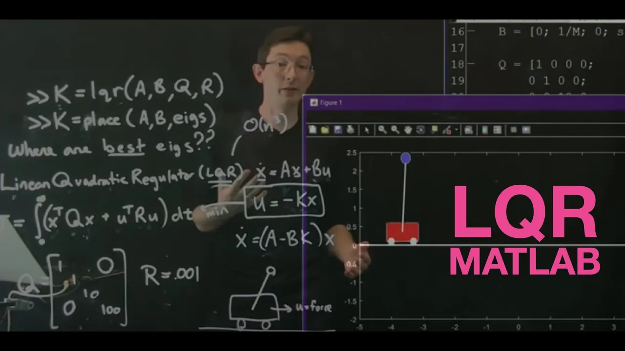
13:03
LQR Control for the Inverted Pendulum on a Cart: Full-State Design
@Eigensteve
243.5K views•2017-01-29

30:32
Ultrasonic Transducers: Resonant Frequency Measurement and Horn Design
@imajeenyus42
229.9K views•2017-02-22

54:16
Polymer Environmental Degradation: Mechanisms & Stabilization
@iit
1.8K views•2012-07-10

33:39
How a Student's Question Saved a NYC Skyscraper from Collapse
@veritasium
22.8M views•2025-04-26
Related Study Plans & Knowledge Roadmaps
Structured learning paths in Engineering
engineering
Building Acoustic Levitators: Physics & Arduino
01The Physics of Sound and Standing Waves
02Piezoelectric Transducers and H-Bridge Drivers
03Arduino Programming: Generating 40 kHz Signals
+ 2 more learning modules
14h5 modules
Explore Roadmap
engineering
Building Peltier Cloud Chambers: Particle Tracks
01Cosmic Rays & Cloud Chamber Physics
02Thermoelectric Cooling (TEC) Fundamentals
03Custom Liquid-Cooling Loop Design
+ 2 more learning modules
18h5 modules
Explore Roadmap
engineering
Yagi-Uda Antennas: Modeling, Build & VNA Test
01Introduction to RF and Antenna Fundamentals
02Yagi-Uda Antenna Design Principles
03Antenna Modeling and Simulation in 4NEC2
+ 2 more learning modules
18h5 modules
Explore Roadmap
engineering
ECG Monitor Design: Op-Amps, Filters & Noise
01Electronics & Breadboard Basics
02Op-Amps and Instrumentation Amplifiers
03Bioelectricity and ECG Fundamentals
+ 2 more learning modules
18h5 modules
Explore Roadmap