Yagi-Uda Antennas: Modeling, Build & VNA Test

Learning Goal: Design, simulate, and construct a directional Yagi-Uda antenna for the 2.4 GHz Wi-Fi band, utilizing antenna modeling software to calculate optimal element spacing, fabricating the physical array, and characterizing its performance using a Vector Network Analyzer (VNA) to measure return loss and directional gain.

---

Prerequisites & Requirements

• Basic Electronics & Physics: Familiarity with high-frequency alternating currents, electromagnetic waves, and basic vector math.
• Software Tools: A computer running Windows (or using wine/virtualization) to run 4NEC2 or MMANA-GAL antenna simulation software.
• Hardware Tools:
  • A portable Vector Network Analyzer (such as a NanoVNA-H or NanoVNA V2) operating up to at least 3 GHz.
  • Solering iron, solder, wire cutters, caliper, ruler, and a drill.
• Materials: Rigid brass/copper wire (approx. 1.5mm to 2mm diameter), square or round wood/plastic dowel for the boom, an SMA female connector, and a 50-ohm coaxial pigtail cable.

---

Estimated Total Study Time

• Theoretical Study & Simulation: 6–8 hours
• Physical Fabrication & Matching Network Build: 4–6 hours
• VNA Calibration, Tuning, and Testing: 4 hours
• Total: 14–18 Hours

---

Module 1: Introduction to RF and Antenna Fundamentals

This module establishes the core mathematical and physical principles of Radio Frequency (RF) systems. You will learn how electric charges convert to propagating electromagnetic fields, calculate wavelength at 2.4 GHz, and understand impedance mismatches, Return Loss, and Voltage Standing Wave Ratio (VSWR).

Why this video

This video is a comprehensive academic introduction to antenna theory. It explains antennas as transducers that bridge guided waves (coaxial lines) to free-space propagation. It covers fundamental concepts of impedance, radiation resistance, and the mechanisms of wave generation, which are critical for understanding how a Yagi-Uda driven element couples energy to the air.

---

Why this video

This video frames electromagnetic radiation in the context of the 2.4 GHz ISM band. It covers how oscillating electrons create electric and magnetic fields, signal attenuation, polarization, and how isotropic antennas compare to directional arrays. It is highly specific to the 802.11 Wi-Fi standard.

---

Why this video

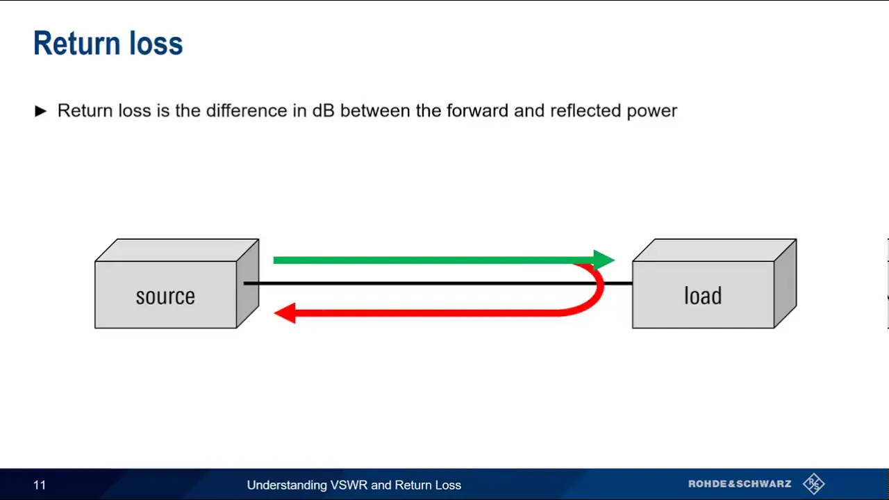
This high-production Rohde & Schwarz tutorial provides a flawless explanation of transmission line reflections, VSWR, and Return Loss. Understanding the mathematical relationship between the reflection coefficient ($\Gamma$), return loss ($RL$), and VSWR is essential for analyzing VNA measurements in Module 5.

---

Module 1 Knowledge Checkpoint

• Calculate the free-space wavelength ($\lambda$) for the center of the 2.4 GHz Wi-Fi band (2.44 GHz) using the speed of light formula ($c = f\lambda$).
• Explain why a standard coaxial transmission line has a characteristic impedance ($Z_0$) of 50 ohms and what happens to signal energy when it meets a load impedance of $100\ \Omega$.
• Convert a VSWR of 1.5:1 to Return Loss (dB) and determine the percentage of reflected power.
• Define polarization and identify the physical orientation required for a Yagi antenna to communicate with a vertically polarized Wi-Fi router.

---

Module 2: Yagi-Uda Antenna Design Principles

This module covers the physics of parasitic elements. You will study how a driven half-wave dipole interacts with slightly longer reflectors and slightly shorter directors to concentrate electromagnetic energy in a single direction.

Why this video

This video uses detailed 3D visual animations to show the phase relationship between the driven element, the reflector, and the directors. It illustrates how the longer reflector acts inductively to push the wave forward, while the shorter directors act capacitively to pull the beam in the direction of fire.

---

Why this video

This tutorial presents the classic physical formulas for calculating the length of each Yagi-Uda component (Reflector $\approx 0.495\lambda$, Driven Element $\approx 0.473\lambda$, Director 1 $\approx 0.440\lambda$) and standard element spacings. It provides a quick design path to sketch out an array before inputting parameters into CAD simulation software.

---

Why this video

This video explains the relationship between the physical length of the antenna boom, the number of directors, and the final directional gain (dBi) of the array. It covers the trade-off between bandwidth, directivity, and feedpoint impedance as elements are added.

---

Module 2 Knowledge Checkpoint

• Explain how a parasitic element, which has no electrical connection to the coaxial cable, receives and re-radiates electromagnetic energy.
• State why the reflector element is placed behind the driven element and why its physical length must be longer than half a wavelength.
• Explain the relationship between element spacing and feedpoint impedance of the driven element. Why does bringing elements closer together lower the impedance below 50 ohms?
• Describe the front-to-back (F/B) ratio of an antenna and specify why a high F/B ratio is beneficial in noisy Wi-Fi environments.

---

Module 3: Antenna Modeling and Simulation

In this module, you will translate physical dimensions into a virtual wire model. You will learn to use Numerical Electromagnetics Code (NEC) software engines to analyze current distributions, evaluate radiation patterns, calculate feedpoint impedance, and run frequency sweeps to optimize the design for the 2.4 GHz band.

Why this video

This practical step-by-step tutorial introduces the interface of 4NEC2, a free-to-use software based on the industry-standard NEC-2 engine. It demonstrates how to establish 3D Cartesian coordinates ($X, Y, Z$), model straight wire elements, define segmentation, assign sources (excitation points), and generate 3D radiation patterns.

---

Why this video

For users seeking a modern or multi-platform alternative to 4NEC2, MMANA-GAL is an exceptional choice. This video presents a quick walkthrough of the MMANA geometry spreadsheet, showcasing how to input wire dimensions, view the 3D geometry, define source segments, and calculate basic S-parameters.

---

Why this video

While focused on a wire dipole variation, this long-form tutorial goes deep into the mechanics of setting up frequency sweeps, plotting SWR curves, and viewing how current distribution behaves on wire segments. This detailed workflow can be applied directly when tuning a 2.4 GHz Yagi-Uda model.

---

Modeling Engine Coverage Note

Simulation Engine Note: Because the video pool lacks a specific tutorial on modeling a 2.4 GHz Yagi-Uda in 4NEC2, you must combine the interface skills from these videos with your manual calculations.

Independent Search Recommendation: If you run into issues modeling high-frequency structures, search for: "4NEC2 wire segmentation limit high frequency" or "MMANA-GAL Yagi optimization tool tutorial". Remember to set wire thickness parameters accurately, as thick copper wire (e.g., 2mm) has a self-inductance that shifts the resonant frequency lower than standard thin-wire calculations suggest.

---

Module 3 Knowledge Checkpoint

• Create a coordinate table ($X, Y, Z$) for a 5-element Yagi antenna operating at 2.44 GHz, defining the driven element center at $(0, 0, 0)$.
• Explain why choosing the correct number of wire segments in NEC engines is critical. What are the dangers of under-segmentation and over-segmentation on the calculation of feedpoint impedance?
• In your simulator of choice, run a frequency sweep from 2.40 GHz to 2.50 GHz. Identify the frequency of lowest SWR and the calculated feedpoint resistance ($R$) and reactance ($jX$).
• Analyze the calculated 3D radiation pattern. What is the simulated gain in dBi, and what is the half-power beamwidth (HPBW) in both the E-plane and H-plane?

---

Module 4: Physical Fabrication of a 2.4 GHz Yagi Antenna

In this module, you will transition from CAD dimensions to physical fabrication. You will calculate velocity factors, cut elements with sub-millimeter accuracy, and assemble a 50-ohm matching network/balun to feed the antenna.

Why this video

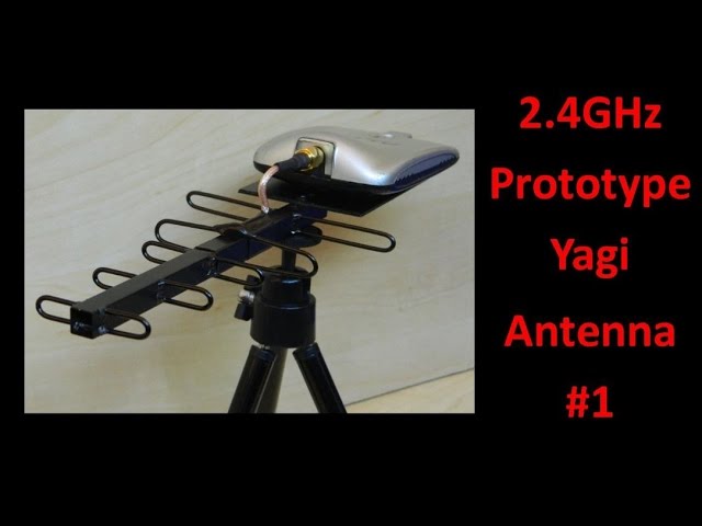
Andrew McNeil is a legendary amateur antenna fabricator. This video demonstrates the step-by-step build of a multi-element Yagi antenna specifically for the 2.4 GHz Wi-Fi band. It covers selecting brass/copper wire, preparing a rigid boom, cutting elements with high physical accuracy, and making direct RF connections.

---

Why this video

A standard Yagi's balanced driven element cannot be directly connected to an unbalanced 50-ohm coaxial cable without experiencing severe shield radiation and impedance mismatch. This video explains the physics and construction of a Gamma Match—an adjustable matching network that steps up the low impedance of a closely spaced Yagi array to match 50 ohms while canceling out parasitic reactance.

---

Why this video

This build video shows an alternative physical construction style, utilizing 3D-printed mounting blocks to secure aluminum or copper element rods to a wooden boom. It highlights the importance of keeping elements isolated from conductive booms if using a metal support system.

---

Fabrication Accuracy Note

High-Frequency Fabrication Warning: At 2.4 GHz, a single millimeter of error in element length or spacing represents approximately 1% of the total wavelength. This can shift the antenna's operating frequency completely out of the Wi-Fi band.

Best Practice: Use digital calipers to measure and cut elements. If you do not construct a physical Gamma Match, you must use a Folded Dipole as your driven element to step up the feedpoint impedance to a workable 300 ohms, combined with a 4:1 coax balun. For a standard split dipole driven element, ensure your coaxial pigtail has a small ferrite bead or a 2-turn coax choke to act as a choke balun.

---

Module 4 Knowledge Checkpoint

• Determine the velocity factor of your chosen solid element material. Adjust your simulated physical lengths to compensate for the velocity factor.
• Describe the physical structure of a Gamma Match: what are the functions of the shorting bar, the gamma rod, and the series tuning capacitor?
• Explain why a non-conductive boom (e.g., wood, acrylic, or 3D-printed PLA) simplifies construction compared to a metallic boom, with reference to element isolation.
• Fabricate your Yagi-Uda array using calipers, securing elements firmly to the boom with epoxy, hot glue, or mechanical brackets.

---

Module 5: VNA Characterization, Tuning, and Measurements

In this final module, you will use a Vector Network Analyzer (such as a NanoVNA) to test, characterize, and tune your fabricated antenna. You will calibrate the VNA, analyze return loss on a Smith Chart, and tune your matching network for optimum performance at 2.44 GHz.

Why this video

A VNA is useless without proper calibration at the exact reference plane where the antenna is connected. This tutorial explains when, why, and how to execute a standard SOLT (Short, Open, Load, Through) 1-port calibration. It guides you in configuring the start/stop sweep frequencies for your Wi-Fi test (e.g., 2.3 GHz to 2.6 GHz).

---

Why this video

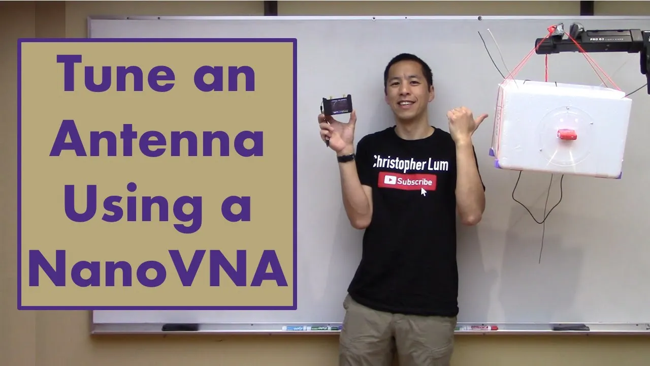
This long-form video walks through the complete hands-on workflow of tuning a real, physical antenna to resonance using a NanoVNA. It demonstrates how to interpret the S11 (logarithmic magnitude) curve to identify the antenna's primary resonance point and how trimming physical lengths shifts the curve.

---

Why this video

Alan Wolke (@w2aew) delivers a masterclass on the Smith Chart and VNA tuning. This presentation explains how to read complex impedance ($R \pm jX$) plotted on a Smith Chart and how to utilize matching components (like series capacitors or shunt inductors) to move the measured point to the center ($50\ \Omega$ pure resistance).

---

Why this video

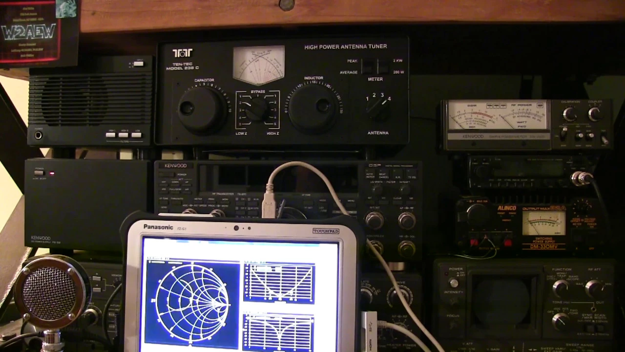
This short, practical follow-up video demonstrates how real-time physical adjustments to a matching network instantly alter the Smith Chart sweep. It provides the visual intuition needed to adjust the shorting bar of your Gamma Match or trim the dipole elements.

---

Module 5 Knowledge Checkpoint

• Calibrate your NanoVNA for a 1-port ($S_{11}$) measurement over the frequency range of 2.3 GHz to 2.6 GHz, utilizing the SMA calibration kit.
• Connect your fabricated 2.4 GHz Yagi. Locate the minimum point on the $S_{11}$ trace. Record the resonant frequency and its minimum Return Loss in dB.
• Open the Smith Chart display format. Identify if your antenna is inductive (upper half of chart) or capacitive (lower half of chart) at 2.44 GHz.
• Step-by-step Tuning: If the resonant frequency is too low, explain why trimming the driven element length or adjusting the matching network shifts resonance higher. Execute tuning until a VSWR of < 1.5:1 is achieved across the 2.4 GHz Wi-Fi band.

---

Course Map

Below is the recommended learning progression path. Note how theory and simulation must occur before physical material fabrication to avoid wasted effort and material.

---

Key People Index

• Dr. Hidetsugu Yagi & Dr. Shintaro Uda: Japanese researchers who co-invented the directional Yagi-Uda array in 1926 at Tohoku University. Uda did the primary design work, while Yagi commercialized and popularized the design globally.
• Phillip H. Smith: An American electrical engineer who invented the Smith Chart in 1939 while working at Bell Telephone Laboratories. His chart remains the premier graphical method to visualize high-frequency transmission line matching.
• Alan Wolke (W2AEW): A prominent RF Design Engineer and popular YouTube educator who specializes in making complex test instrument operations, analog circuits, and VNA measurements highly accessible.
• Andrew McNeil: An expert amateur antenna designer and videographer who has spent decades creating, optimizing, and teaching low-cost, high-performance DIY microwave and Wi-Fi antenna construction.

---

Final Self-Assessment

Complete this comprehensive checklist after completing all lessons, simulations, and builds to verify that your antenna meets the standard RF requirements for deployment.

• Mathematical Verification: You have calculated free-space wavelength ($\lambda \approx 12.3\text{ cm}$ at 2.44 GHz) and adjusted your physical element lengths based on the velocity factor of your copper/brass wire.
• Simulation Completion: You successfully created a multi-element (minimum 3-5 elements) wire model of your 2.4 GHz Yagi-Uda antenna in 4NEC2 or MMANA-GAL.
• Impedance Matching Design: Your simulation confirms a calculated real impedance ($R$) close to $50\ \Omega$ and a reactance ($jX$) close to $0\ \Omega$ at the center frequency, or you have integrated an adjustable physical matching network (like a Gamma Match).
• Precision Fabrication: Your physical antenna has been built using a digital caliper to verify that all element lengths and spacings are within $\pm0.5\text{ mm}$ of the calculated design values.
• Unbalanced Current Choking: Your feed line features a functional balun or ferrite choke to prevent RF shield currents from radiating along your coaxial feedline.
• VNA Calibration: You executed a fresh 1-port SOLT calibration on your NanoVNA, ensuring the calibration plane matches the exact connection point of your antenna feed line.
• Return Loss Characteristic: The tuned antenna registers an $S_{11}$ Return Loss of $-15\text{ dB}$ or lower (corresponds to a VSWR of 1.43:1 or lower) at 2.44 GHz.
• Smith Chart Verification: When viewing the center of the Wi-Fi band on the VNA Smith Chart, the trace marker is centered near the intersection of the pure-resistance line ($50\ \Omega$) and the zero-reactance horizontal axis.
• Directional Field Test: When orienting the physical antenna, a nearby Wi-Fi router's Received Signal Strength Indicator (RSSI) significantly increases when the front directors point at the source and drops when rotated 90 degrees or when pointing backward (demonstrating directional gain and front-to-back ratio).