






















RF signals propagate as electromagnetic waves with horizontal magnetic and vertical electric field components, where signal strength follows a logarithmic dB scale (adding 3dB doubles power, adding 10dB increases power tenfold); antennas focus signals through gain, with reciprocity meaning transmit and receive patterns are identical, and higher gain antennas achieve greater range but narrower coverage, while link budget calculations incorporating EIRP, fade margin, and factors like multipath, Fresnel zone clearance, and frequency-dependent attenuation determine overall wireless link performance.
RF and Antenna Fundamentals for 802.11 Networks
Added:Basic understanding of electromagnetic wave properties, including frequency, wavelength, and the RF spectrum.
Familiarity with the OSI model, particularly the Physical (PHY) and Data Link (MAC) layers in networking.
Fundamentals of logarithmic math and decibel calculations (dB, dBm, dBi) used to measure signal strength.
Basic electrical concepts such as power, voltage, impedance, and signal attenuation.
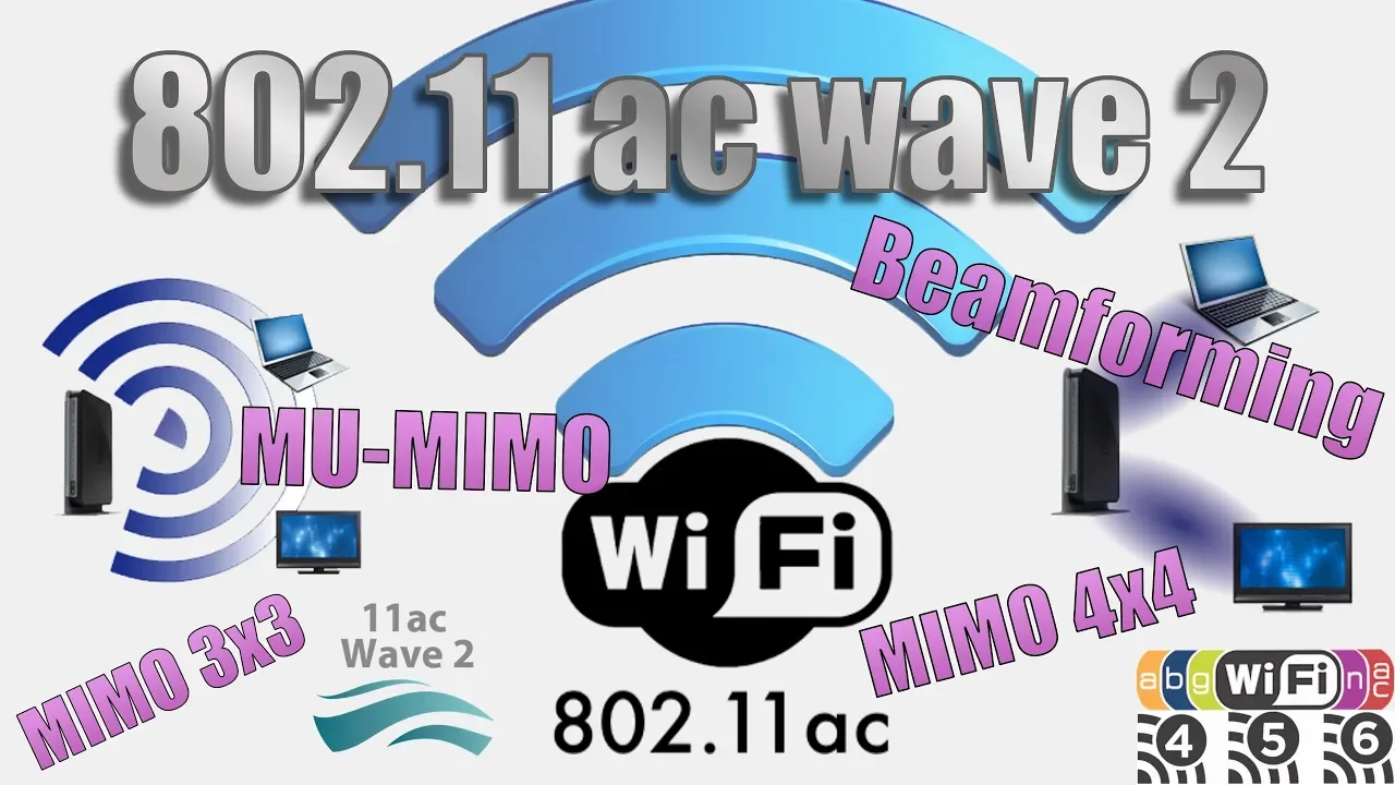
Advanced wireless technologies like MIMO (Multiple-Input Multiple-Output), transmit beamforming, and MU-MIMO used in modern Wi-Fi standards (802.11ac/ax/be).
Practical wireless site surveying, heatmapping, and RF deployment planning using industry-standard tools.
RF spectrum analysis to identify, troubleshoot, and mitigate non-Wi-Fi interference and channel congestion.
Designing and calculating complex link budgets for outdoor, long-range Point-to-Point (P2P) and Point-to-Multipoint (P2MP) wireless bridges.
138.5K views2.8Klikes39:05Original Release: 2015-09-17
Hi, this is Hank Audi. Thank you for watching. This webcast will cover the basic properties of RF and antennas with a slight focus on the 802.11 protocol.
Prior RF knowledge is not required. We will start by discussing how signal is sent and received. Once we have a good idea of how signal propagates as waves, we will discuss a certain property of the waves called polarity.
signal is measured in units of decibb or dB. The dB scale is logarithmic. We will use some simple tools to better understand how this scale works. EIRP or equivalent isotropically radiated power is a quantity of RF systems that typically comes into play when considering laws pertaining to the transmit power of radio transceivers.
We will then discuss how the field strength of a signal can change at different orientations with respect to the transmitting antenna. Generally speaking, there are three types of antennas used in 802.11 wireless systems.
Omniirectional, sector, and directional antennas. We will see how each of these differs from the rest. Antennas have several aspects that need to be considered when designing an RF system. First is typically gain which is closely related to signal spread.
Reciprocity states that an antenna not only focuses outgoing signal from the transceiver but also focuses incoming signal to the transceiver. Antennas heavily influence the range between two RF devices. We'll discuss how using various antennas can achieve different ranges. The mounting of the antennas can have a substantial influence in the performance of the system. We will see how to achieve optimal results by appropriate antenna mounting. Enemies of signal quality come in many different forms. Multipath is essentially an echo of the transmitted RF signal. Obstructions are anything that can block the signal between two RF devices. The Fresnel zone is a mysterious effect that weakens signal as the line of sight between two IO devices is encroached upon. Weather can weaken a signal as well. But if RF systems are designed appropriately, the negative effects of weather can be overcome. Interference can have a devastating effect on RF systems regardless of which end of the link it is affecting. The RF noise floor is basically an ambient noise in the location of the RF system. The louder this ambient noise, the more trouble the system will have in communicating.
The VSWR or voltage standing wave ratio is a property of antennas and can have multiple negative effects if its value is too high. The connectivity of a link refers to the rate of data sent in one direction. Transmit power and receive sensitivity both play a significant role in the range of a link and can actually depend on the connectivity of the link.
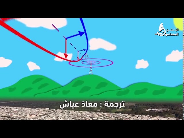
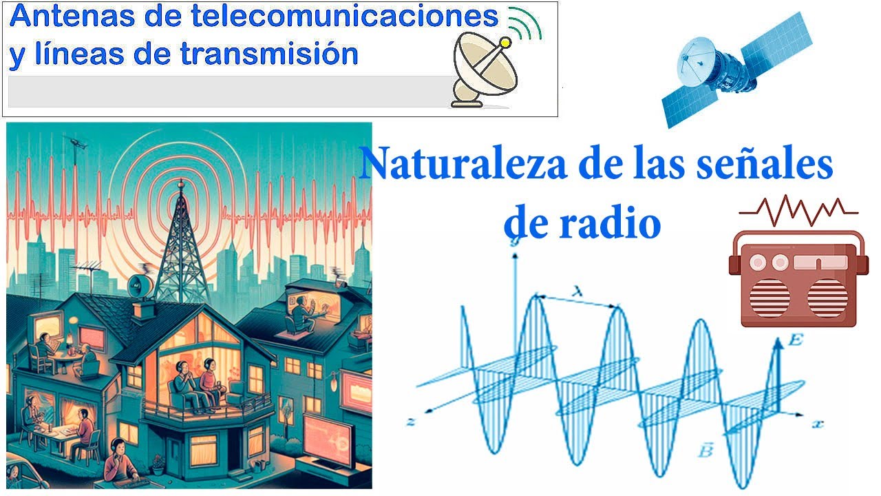
Connectivity and throughput are two different quantities and it is very important to distinguish between the two when estimating the capacity of a network. Since connectivity affects both transmit power and receive sensitivity, it heavily influences how much range a link can achieve. Link budgets take into account everything that is involved in sending and receiving the signal. Signal passes through cables and connectors. It is focused by antennas and attenuated by the air through which it passes. The fade margin basically refers to how much the link is overengineered. Finally, we will explain that greater range will give greater attenuation. As the illustration shows, signal is generated by electrons oscillating in a piece of metal. This is referred to as a dipole and is basically a single antenna element. As per the right-h hand rule, if the electrons are moving in the direction the thumb is pointed, a magnetic field is generated around the piece of metal in the direction the fingers are pointed. Here we have a visual interpretation of what was stated on the previous slide. We can see as the electrons move up and down, the magnetic field around the wire changes directions from clockwise to counterclockwise. The oscillating magnetic field induces movement of electrons and other metal objects in a direction perpendicular to the magnetic field. What is going on here is that this oscillating magnetic field produces a corresponding perpendicular electric field. When the magnetic field changes directions, the electric field changes directions. When this oscillating electric field hits electrons in other metal objects, it forces those electrons to oscillate as well. Here we see the system as a whole which includes the transmitting antenna element and the receiving antenna element. The electrons in the transmitting antenna element are oscillating vertically which generates an oscillating magnetic field in the horizontal plane. This magnetic field generates an electric field oscillating in the vertical plane. This vertically oscillating electric field hits the receiving antenna element and forces its electrons to move up and down.
It can be seen that there is a slight lag between the movement of electrons in the receiving antenna element and the electrons in the transmitting antenna element. This is due to the fact that the effect does not happen instantaneously. The waves do travel at the speed of light. So the time is not much but it does take time nonetheless. In the interest of looking from a different point of view, we are viewing the same system from the top. It can be seen that the effect propagates outward from the transmitting antenna.
The magnetic field changes directions and eventually hits the receiving antenna. As mentioned before, the signal propagates as a wave with a horizontal magnetic field component and a vertical electric field component. The electric field component of the wave is the component of interest. As can be seen, when the transmitting antenna is vertical, the electric field is vertical. In the lower part of the illustration, the transmitting antenna is horizontal, which dictates that the electric field is also horizontal. This is the polarity of the antenna. We will now discuss how changing polarities can affect the receive signal strength. In this situation, both the transmitting and receiving antenna are vertical. This results in receiving a full signal strength. As the receiving antenna is tilted sideways, the vertical electric field wave cannot influence the electrons inside the receiving antenna as much as when it was vertical. This results in a decrease of received signal. When the receive antenna is completely horizontal, the electric field waves have no influence on the electrons inside the receiving antenna element. the electrons are effectively getting pushed against the ceiling and against the floor of the receiving antenna element. In other words, there will be no movement of the electrons inside the antenna element and the signal will not be received at all. Signal is measured in units of dd or decb. The power of a signal along a conductor, which could be a pigtail inside of an enclosure or an RF cable that is going to an antenna, is typically referred to as DBM or decibb relative to 1 matt. The power of signal propagation through the air is generally referred to as di or dB relative to an isotropic radiator. An isotropic radiator is one that emits signal equally in all directions. The sun is a good example of this. This is not theoretically possible in RF and we will discuss this shortly.
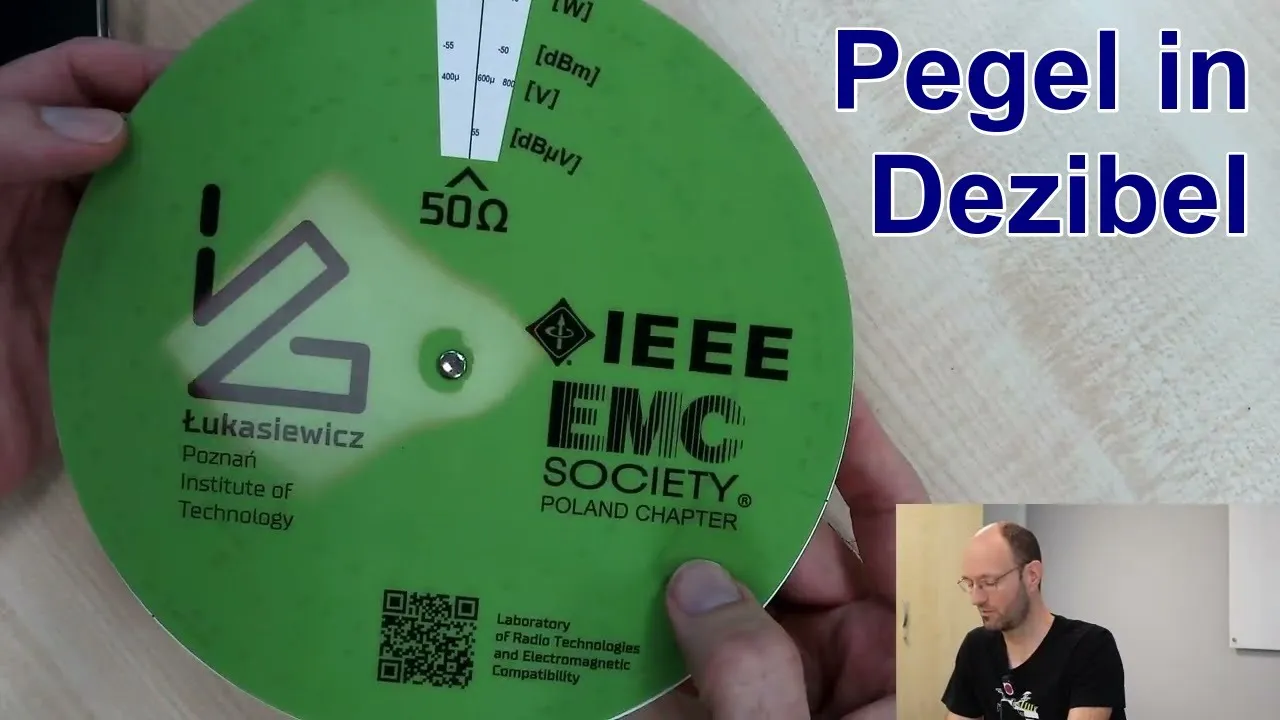
But for measurement purposes, we use an isotropic radiator as a reference. The decibel scale is logarithmic. There are two rules of thumb to conveniently remember the power to dB conversion. The first rule of thumb is adding 3dB doubles the power.
If we take a look at the numbers here, it can be seen that every time 3dB is added, power doubles. The same goes in reverse. As 3dB is taken away, power is cut in half. The second rule of thumb is adding 10 dB to an RF system will increase its power by a factor of 10. This goes in reverse as well. Taking 10 dB away from an RF system decreases the power by a factor of 10. Taking the two rules of thumb that we know, let's do an example.
Let's find the power of 28 dBm. Let's start with 40 dBm, which equals 10 watt. Now, let's take 3dB away to cut the power in half. We will take another 3dB away and cut the power in half once again.
We will continue to do this until we eventually reach our goal of 28 dBm which equals 625 m. Now let's consider 19 dBm. Looking at the information to the left, we can see that 29 dBm equals 800 m. We also know that taking away 10 dB from a system will decrease its power by a factor of 10 and in this case gives us our answer directly of 80 m. Keep in mind that these are just rules of thumb and not exact but accurate enough for quick off the top of the head calculations. As previously mentioned, an isotropic radiator emits signal equally in all directions. Here we have two isotropic radiators. The one on the left is being supplied with 20 dBm of power. The one on the right is being supplied by twice the power or 23 dBm. An antenna can focus the signal from a weaker transmitter to the same strength as a 0dbi isotropic radiator with a stronger transmitter. Looking at the two systems below, we can see that the one on the left has much more power than the one on the right.
However, the directional antenna on the right compensates for the lower power.
This gives both systems the same equivalent isotropically radiated power. In converting the dB of the two systems into millows, we can see just how much more powerful the system on the left is as compared to the system on the right. This is testament as to how strategic antennas are in designing RF systems.
Now we will discuss why isotropic radiators are not theoretically possible. Here we have a single antenna element and an electron that it is affecting. The electron is a distance away and it sees the antenna element at a big angle. Therefore, the electron experiences a strong field strength.
As we change the orientation of the electron but keep the same distance, we can see that the electron now sees the antenna element at a small angle, therefore experiencing a weak field strength. Now we position the electron directly above the antenna element, but keep the same distance. It can be seen that the electron sees the antenna element at a zero angle, therefore experiencing a zero field strength.
This effect of field strength versus orientation results in the illustrated field strength pattern. Please note that only one side of the field strength pattern is drawn. In actuality, the pattern takes the shape of a donut or a Taurus around the antenna element. Now we will discuss how waves are used to shape signal. Here we have two antenna elements, one directly above the other and separated by a distance. The two elements will generate waves. At some orientations, the waves will cancel each other out. At other orientations, the waves will compound each other. As the waves propagate outward, it can be seen that the green lines indicate where the waves compound each other.
Looking closely, it can be seen that the red lines indicate exactly where the waves cancel each other out. The overall effect of the waves combining with each other produces a primary lobe and two secondary loes around the antenna elements. Now we will discuss types of antennas. Although there are several different types of antennas on the market, generally speaking, 802.11 systems use omniirectional antennas, sector antennas, and directional antennas. Let's take a look at omniirectional antennas. Here we have some signal strength graphs for three different antennas. The first graph on the bottom left represents a single element antenna. The three-dimensional Taurus shape of this graph is illustrated at the top left.
The bottom center graph illustrates a dual element antenna. This is the same pattern that was just described by two waves combining with each other. The three-dimensional version of this graph is illustrated at the top right. The bottom right graph represents several antenna elements. It can be seen that the more elements that are added, the more elongated the primary lobe gets.
This is effectively increasing the gain or the focus of the antenna.
Antennas are described in industry as having a vertical signal spread.
However, it can be seen that the signal falls off gradually as the angle increases from the horizontal and decreases from its strongest point. In other words, there is no definite angle where the signal drops suddenly. Vertical signal spread is defined as the angle at which signal falls off 3 dB from the strongest point.
On this graph, the concentric rings represent 10 dB each. We can estimate that the -3dB mark is about 20° above and below the horizontal and that the vertical signal spread for this antenna is 40°. When considering the pattern of a dual element antenna, we can see that the primary lobe becomes more elongated, therefore giving it a smaller vertical signal spread. Here we have graphs and illustrations of the signal spread from a sector antenna. Sector antennas are basically omnidirectional antennas with reflectors behind them. The shape of the reflector influences the angle of the sector antenna's horizontal signal spread. This particular sector antenna has a vertical signal spread of 15° and a horizontal signal spread of 90°. Directional antennas have extremely elongated primary loes. They also have numerous secondary, tertiary, and quatinary loes.
The gain of an antenna refers to the degree of focus it gives the power supplied to it. This typically ties directly into its signal spread. Looking at the two signal patterns illustrated below, we can see that the top signal pattern has a vertical spread of 24° and a corresponding gain of 8 dBi. The signal pattern on the bottom has a vertical spread of 12°, which gives it twice the focus as the signal spread on the top. Since the focus is doubled, it effectively doubles the radiated power at the horizontal orientation. Since the radiated power at the horizontal is effectively doubled, this implies that the gain of the antenna, which is measured in dbi, is increased by three, giving the antenna on the bottom a gain rating of 11 dBi. Here we have a similar example except with sector antennas. The sector antenna on the left has a horizontal beam width of 30° and a vertical beam width of 20° and an overall gain of 15 dBi. The sector antenna on the right has a horizontal beam width of 15° and a vertical beam width of only 10°. Its gain is 21 dBi. We're doubling the focus increases the gain by 3 dBi. Four times the focus increases the gain by 6 dBi. Antenna's focus signal. They also narrow the field of view of the RF they receive. Here we have an analogy where an eye is looking at a distant candle and it sees the candle quite dimly. Down below we have two radio transceivers, one transmitting and one receiving. Each has a low gain omniirectional antenna.
So the signal between the two is quite weak. If the eye were to look at the distant candle through a telescope, the eye would be blinded by the light coming from the candle.
If we mount a high gain directional antenna on the receiving radio transceiver, it would take the weak signal propagated from the distant low gain omniirectional antenna and heavily focus the signal into the receiving transceiver just as the telescope did with the eye. In fact, reciprocity dictates that this link is 100% symmetrical. In other words, considering that the transmit powers are equal on both ends of the link, the received signals at each end of the link are also equal. Let's look at reciprocity from a different perspective. In this situation, the mid gain antenna has a wide field of view and the high gain antenna has a very narrow field of view.
Considering that the mid gain antenna has a wide field of view, it does not see much of the candle. However, the high gain antenna with a very small field of view is zoomed in on the candle and therefore sees it very brightly. Here is yet another example of how a higher gain antenna can focus or amplify an incoming signal to the receiving transceiver. The wave is received by each antenna element. The more antenna elements there are, the more signal is sent to the receiving transceiver. The range between two devices is a popular question in RF and it depends on several things. Here we will discuss how antennas influence range. It is important to note that the antennas on each end of the link influence the overall range. In the case of omnidirectional to omniirectional, the range will not be too substantial.
Exact range numbers are intentionally being left out for now, but we will elaborate more on that a bit later. If one of the antennas below were replaced with a directional antenna, the link would be able to achieve a much longer distance. If both of the antennas below were replaced with directional antennas, the link would be able to achieve a huge distance.
RF devices can be equated to mouths and ears. Just as RF devices transmit and receive, our mouths talk and our ears listen. If we are having a conversation with a person and we start talking louder, we could stand further away and the person would still be able to hear us. This is analogous to a transceiver transmitting at a higher power.
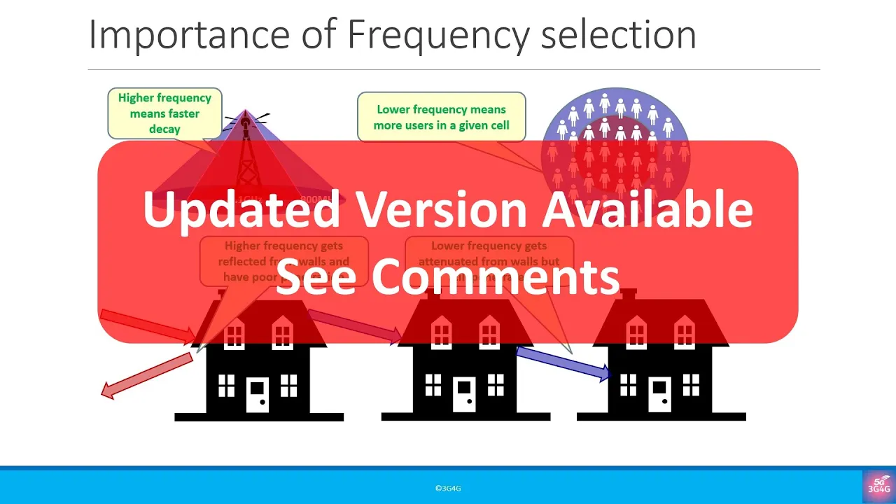
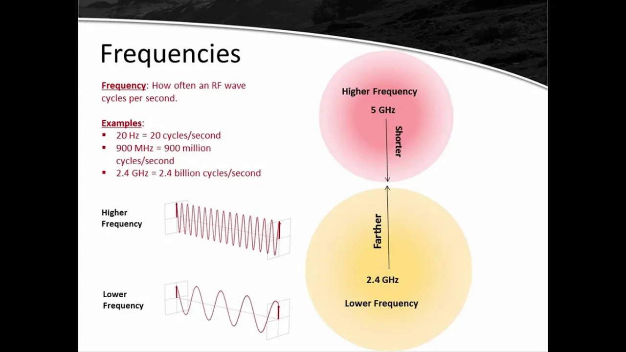
Similarly, if the person we are talking to suddenly acquired hyper sensitive hearing, they would be able to stand further away and still be able to hear us. This is analogous to a transceiver having a higher receive sensitivity. Another aspect of RF that influences range is the frequency of the link. For example, 2.4 GHz propagates about twice as far as 5 GHz.
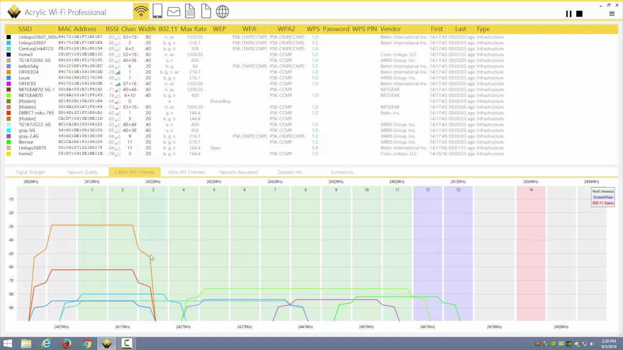
900 megahertz propagates about five times farther than 5 GHz. This may vary a bit, but is usually a good rule of thumb. As mentioned before, antennas are typically composed of a pattern of dipole radiators. This gives them their unique signal spreads. It also influences how we mount antennas. Considering that antennas generally have a zero field directly above and below, this is the ideal place to mount other antennas. Even slightly offsetting antennas that are mounted directly above and below each other will put each antenna in the others side lobes. This can negatively affect the performance of each antenna. This is not such a concern if the antennas are on different frequency bands such as 2.4 GHz and 5 GHz. However, if for example, one antenna was on 2.4 GHz channel 1 and the other was on 2.4 GHz channel 6, there could potentially be interference between the two antennas. The reason for this is although 2.4 GHz has three non-over overlapping channels, it can be seen in the illustration below that the channel masks do overlap if the received signal is high enough.
Multiath is essentially an echo of an RF signal. Here we have the simplest case of multipath. However, with numerous reflective surfaces around an RF link, it is possible for the multiath effects to become very complicated and impossible to predict.
One way to combat multipath is to move one of the transceivers. Just as inching forward in your car at a stoplight helps the radio station come in better. Simply moving either of the involved transceivers can improve the performance of the link if multipath is suspected.
Changing the channel of the link can also help as different channels have different wavelengths and therefore different multiath effects. When deploying RF systems, it is important to consider any future obstructions that may come in the line of sight between any two RF devices involved in a [Music] link. The Fresnel zone is the immediate volume around the line of sight between two antennas. When obstructions encroach upon the frenel zone, the link can become weakened even if the line of sight is not blocked by the obstructions. Here we can see exactly how the signal becomes weakened by the nearby obstruction. The wave is grabbed by the obstruction and gets stretched and weakened as it propagates towards its destination antenna.
The Fresnel zone not only grows with lower frequencies but also with longer distances. Here are some examples of Fresnel zones and corresponding frequencies. Weather does affect signal strength and as we will see later it is good practice to overengineer RF links so that the negative effects of weather are minimized.
Interference in RF is an unavoidable headache and often stems from external sources. When designing RF systems, it is important to do a pre-scan of the area in order to determine if any interference exists on the channels of interest. As we will see, interference on either end of an RF link will affect the link as a whole.
Many packets transmitted in the 802.11 protocol require the receipt of any acknowledgement packet which is sent from the receiver. The acknowledgement packet is required before the next packet is sent. If the acknowledgement packet is not received after a period of time, the original packet is resent. Here we see how interference at the receiving antenna can affect the link as a whole. The initial packet is sent and the acknowledgement packet is received. However, when interference happens at the receiving antenna, the initial packet is not heard. Therefore, the acknowledgement packet is not sent and the link as a whole will fail. Now, we consider what happens when interference affects the transmitting antenna. The initial packet is sent and successfully received, but the acknowledgement packet is not heard by the transmitter. Therefore, the initial packet is reset. Again, the link as a whole fails. The noise floor is the background noise for RF. When considering audible noise, this could be compared to the ambient noise in a restaurant. Any signal at or below the noise floor will not be receivable. The signal to noise ratio or SNR compares the power of the receive signal to the power of the noise floor.
A typical noise floor in an RF environment might be around 94 dB. A typical signal might be around 74 dB.
This gives an SNR of 20 dB. Antennas come with a rating of VSWR or voltage standing wave ratio. A high VSWR which may be considered greater than 2.0 zero can result in a weaker transmitted signal. In some cases, a high VSWR can cause damage to the transmitter. In the situation below, we have an RF cable attached to an antenna and a water channel. As can be seen, the water waves flow freely through the channel. If the antenna does not have a high VSWR, the RF waves will also flow freely through the system.
Now let's take a look at what happens when the antenna is replaced with one that has a high BSWR. In the case of the water channel, it is as if the channel was narrowed, which allows only part of the wave to pass. This results in a weakened transmitted signal. In addition, part of the wave is reflected backwards, which can potentially cause damage to the transmitter.
A radio transceiver involved in a link will strive to achieve the maximum possible connectivity of the medium. Links are formed from beacons being sent out so that other RF devices are aware that a link is being offered.
Beacons are sent out at the lowest rate of the medium. This is the rate at which links are initially formed.
After a link achieves successful transmissions at the lowest connectivity or data rate, it will attempt transmissions at the next highest connectivity. If success is again achieved, the link will jump to the next highest connectivity and so on. If after jumping to a higher connectivity, the link experiences unsuccessful transmissions, the link will back down to the lower connectivity.
as an aspect of the transmitter.
Transmit output power depends on the connectivity at which the radio is transmitting. The example given here is for 5 GHz 802.11a. As can be seen, the higher connectivities actually have a lower transmit power than the lower connectivities. as an aspect of the receiver. The receive sensitivity also depends on the connectivity of the signal that the radio is receiving. This example is also given for 5 GHz 802.11a. What can be seen here is that the receiver actually needs to receive the higher connectivities at a higher power in order to interpret them. This graph takes into consideration the last two aspects described. Higher connectivities not only need to be received at a stronger signal in order to interpret the modulation, they are also transmitted at a lower power. These combined effects result in high connectivities having much shorter lengths. On the other hand, lower connectivities transmit at a much higher power. They're also received with a very high sensitivity. These combined effects result in lower connectivities being able to achieve much longer links.
Please note that the graph below uses fixed yet arbitrary values for antenna gain. Only transfer power and receive sensitivity that correspond to the respective connectivities were changed. It is important to distinguish between connectivity and throughput especially when it comes to managing customers expectations of network performance. Connectivity refers to the data rate in one direction of a link.
TCP IP throughput requires the acknowledgement packet mentioned before.
This makes throughput a two-way street. To give an example of the difference between connectivity and throughput, here are the values of connectivity for 802.11a and their corresponding approximate throughput values. When considering 802.11n, the values for connectivity and throughput can be much greater.
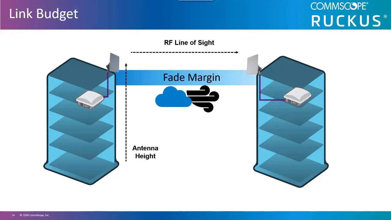
Radio cards are small electronic devices that are responsible for transmitting and receiving the signal through the antennas. They add transmit power or gain to the link budget. As the signal travels through pigtails and antenna cables, there is a slight decrease in signal. Therefore, loss is added to the link budget. Antennas add gain to the link budget. In this example, a total of 31 dBi is added. The signal will attenuate over distance. This is comparable to the walls of a balloon getting thinner as it expands. This is called free space loss.
Free space loss is frequency dependent.
The higher the frequency, the greater the loss. A link is usually designed to allow for unexpected loss that may occur. This is done with appropriate transmit powers, antenna gains, and cable runs. This is the overengineering of the link we were talking about earlier. The fade margin is the strength of the received signal over the strength of the desired signal. In the example given, the received signal is 56 dB. The desired signal is -74 dB. Recall that this is the signal needed in order to achieve maximum connectivity in the 802.11a protocol. The difference in these two values gives us our fade margin of 18 dB. In summary, we started out by seeing how signal is sent and received. We discuss how electrons that are oscillating in a metal wire which represents the transmitting antenna will generate a surrounding magnetic field around the wire. This magnetic field changes directions as the electrons do.
The alternating magnetic field has a corresponding perpendicular electric field. This outwardly propagating electric field affects electrons in other metal objects. The result is that the electrons in the receiving antenna elements mimic the electrons in the transmitting antenna elements. Polarity is simply the orientation of the electric field. When the transmitting antenna element is vertical, the electric field is vertical. When the transmitting antenna is horizontal, the electric field is horizontal. The measurement of signal is on a logarithmic scale. Two rules of thumb that help us to convert dB to power or millows are the following.
Adding 3dB doubles the power and adding 10 dB increases the power by a factor of 10. EIRP or equivalent isotropically radiated power is an important parameter in abiding by the laws pertaining to the transmissions of RF systems. It states that a transmitter and an associated antenna cannot exceed the radiated power of a system that has the same total power when assuming a zero gain antenna. There are typically three types of antennas used in 802.11 systems.
Omniirectional, sector, and directional.
Each uses different numbers and arrangements of antenna elements or different shaped reflectors to focus the signal. Increasing the focus of the signal coming from an antenna can be referred to as increasing the gain of the antenna. The tighter the focus, the higher the gain. Reciprocity states that antennas not only focus signal being sent from the transmitter but also focus incoming signal to the receiver. Antennas on each end of the link heavily influence range. A link can achieve much greater range with use of higher gain antennas. Antennas should be mounted such that they do not interfere with each other. This comes into play particularly when two antennas are using channels that are adjacent on the RF spectrum. Multipath is essentially an echo of an RF signal. Multipath situations can become extremely complicated and impossible to predict.
The first step in combating multipath is to simply move either RF device involved in the link, even if it is just a few feet. Changing channels can also affect multipass situations. Obstructions can hinder links or kill them altogether. When deploying an RF system, it is important to consider what obstructions may come in the line of sight of a link in the future. Obstructions that impinge upon the fresnel zone can severely weaken a link without even blocking the line of sight. This is done by the obstruction grabbing the RF wave and stretching it as it propagates farther, which causes the received signal to become much weaker. The lower the frequency, the larger the frenel zone radius. Weather does affect RF signals, but systems should be designed to be strong enough to overcome the effects of weather. Interference can stem from many different external sources. The deployment area of an RF system should be scanned appropriately before deployment so that clean channels can be identified. Recall that interference on either end of an RF link can affect the link as a whole. The noise floor in an RF environment can be compared to the ambient noise in a real life situation such as being at a crowded restaurant or standing near a waterfall. The signal to noise ratio is the power of the receive signal over the noise floor. If the noise floor is too high, the signal will not be able to be interpreted. This would compare to being at a jam-packed sports arena with the person sitting next to you whispering. Most likely, you would not be able to interpret the whispering. The voltage standing wave ratio is a property of antennas that need to be considered in order to ensure the outgoing signal leaves the transmitting system smoothly. If the VSWR is too high, this will both weaken the transmitted signal and cause reflections back into the transmitter, which can potentially cause damage. The radio card is a small device that is responsible for sending and receiving the signal. When links are initially formed, the radio cards will strive to achieve the highest possible connectivity. At the highest connectivity, the transmit power starts to decrease. In addition, the receive sensitivity also starts to decrease.
This results in links being able to achieve much greater distances at lower connectivities. Connectivity pertains to data flowing in one direction.
Throughput takes into account data that may require acknowledgement packets and is therefore a two-way street. The difference between connectivity and throughput is an important aspect when it comes to managing customers expectations of network performance.
Link budgets take into account everything through which the signal passes between the transmitting radio card and the receiving radio card, including transmit power. Link budgets should be designed with sufficient fade margin such that the link is strong enough to withstand unexpected losses that may occur due to weather, weaken RF connectors, or anything else that affects the link budget. Thank you for watching. This has been Hank Audi. Please find me on linkedin.com or leave comments below.
Up Next

3:51
Yagi Antenna Basics Explained: Gain, Directional Patterns & Applications
@RFShop
23K views•2020-03-15

30:32
Ultrasonic Transducers: Resonant Frequency Measurement and Horn Design
@imajeenyus42
229.9K views•2017-02-22

54:16
Polymer Environmental Degradation: Mechanisms & Stabilization
@iit
1.8K views•2012-07-10

33:39
How a Student's Question Saved a NYC Skyscraper from Collapse
@veritasium
22.8M views•2025-04-26
Related Study Plans & Knowledge Roadmaps
Structured learning paths in Engineering
engineering
Building Acoustic Levitators: Physics & Arduino
01The Physics of Sound and Standing Waves
02Piezoelectric Transducers and H-Bridge Drivers
03Arduino Programming: Generating 40 kHz Signals
+ 2 more learning modules
14h5 modules
Explore Roadmap
engineering
Building Peltier Cloud Chambers: Particle Tracks
01Cosmic Rays & Cloud Chamber Physics
02Thermoelectric Cooling (TEC) Fundamentals
03Custom Liquid-Cooling Loop Design
+ 2 more learning modules
18h5 modules
Explore Roadmap
engineering
Yagi-Uda Antennas: Modeling, Build & VNA Test
01Introduction to RF and Antenna Fundamentals
02Yagi-Uda Antenna Design Principles
03Antenna Modeling and Simulation in 4NEC2
+ 2 more learning modules
18h5 modules
Explore Roadmap
engineering
ECG Monitor Design: Op-Amps, Filters & Noise
01Electronics & Breadboard Basics
02Op-Amps and Instrumentation Amplifiers
03Bioelectricity and ECG Fundamentals
+ 2 more learning modules
18h5 modules
Explore Roadmap