
![Rezystancja, reaktancja, impedancja, moc bierna, czynna, pozorna | #98 [Podstawy]](https://i.ytimg.com/vi/X1ulcKR7Ue0/maxresdefault.jpg)















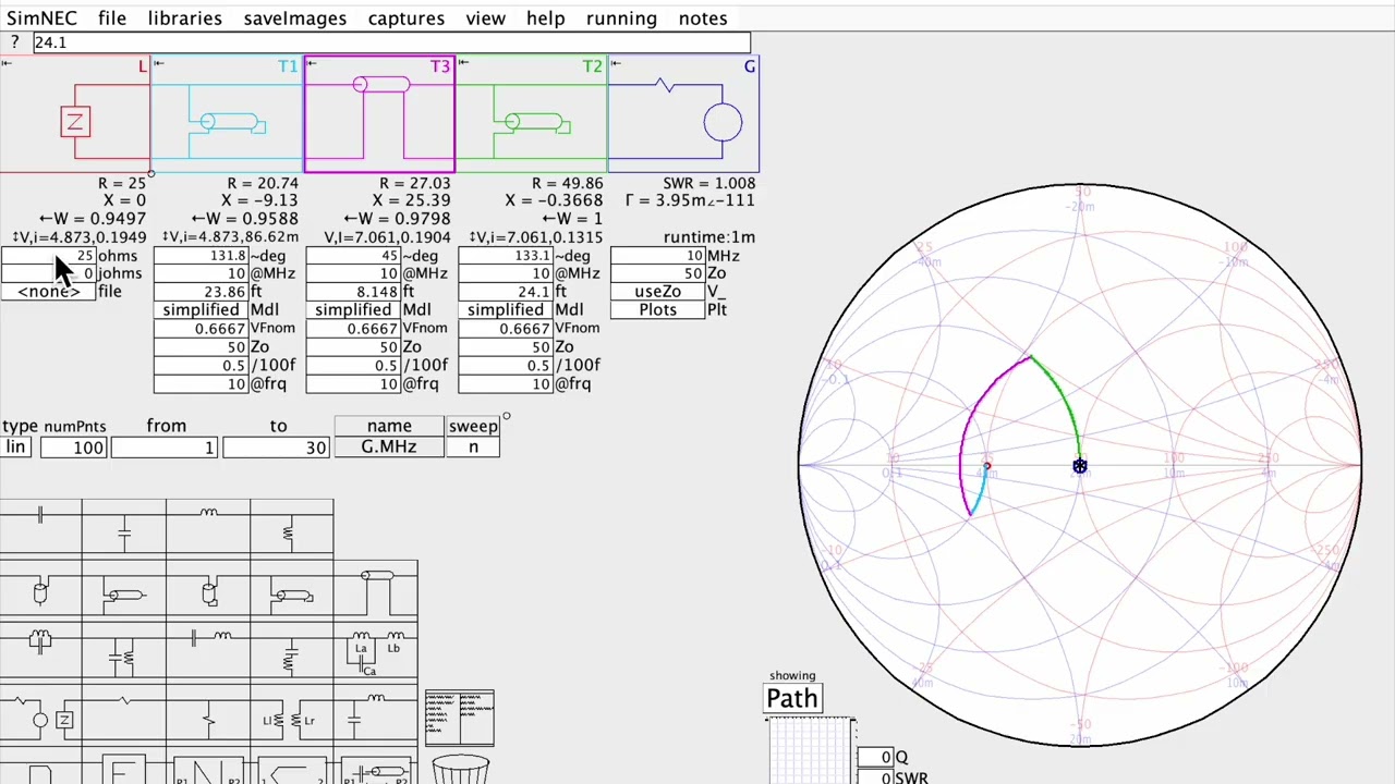





A Smith chart is a graphical tool that plots complex impedance (resistive and reactive components) and enables visualization of SWR, return loss, and transmission line effects; by normalizing impedance to the system impedance (typically 50 ohms), one can analyze antenna performance, design matching networks, and understand how transmission line length affects impedance through rotation on the chart, with minimum SWR occurring at the point closest to the center of the chart.
Smith Charts and the NanoVNA: Antenna Impedance and Matching Network Design
Added:Basic AC circuit theory, including complex impedance (resistance and reactance, represented as Z = R + jX).
Fundamental RF wave propagation concepts, specifically Voltage Standing Wave Ratio (VSWR) and the reflection coefficient.
Basic antenna theory, including resonance, feedpoint impedance, and why impedance matching is necessary to prevent signal loss.
An introductory understanding of Vector Network Analyzer (VNA) operation, particularly how it measures reflection coefficient (S11 parameters).
Advanced lumped-element matching network topologies, such as Pi (π) and T networks, for bandwidth control.
Transmission line matching techniques, including single-stub and double-stub tuning methods on microstrip lines.
Precision VNA calibration techniques (SOLT: Short-Open-Load-Thru) and port extension to de-embed the effects of cables and test fixtures.
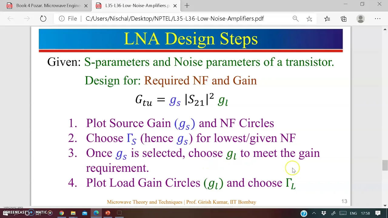
RF amplifier matching design, including the use of constant gain and noise circles on the Smith chart for Low-Noise Amplifiers (LNAs).
40.6K views1.6Klikes54:48Original Release: 2022-02-24
i recently gave a presentation virtually to the san fernando valley amateur radio club w6sd in california and the talk was really a combination of my introduction to smith charts as well as using the nano vna to characterize antennas and kind of combining those two topics together so sit back and enjoy the presentation so we're going to talk a bit about the basics i want to give everybody a basic understanding of what the smith chart is because it actually can be quite useful not only to look at what your antenna looks like and making measurements with it but uh if you're ambitious enough to go you know design a matching network um this can actually help you do that if you enjoy uh kind of you know building things like that that type of thing it's also pretty helpful even if you're using a manual antenna tuner to watch what's going on on the smith chart we'll actually see that here as well so let's get rolling so the first question is you know what is a smith chart and it really is a graphical tool that allows you to plot and compute a number of different things uh first and foremost it allows you to plot complex impedance okay meaning the real or resistive component as well as the inductive or capacitive component of an impedance and any non-resonant you know type of device including an antenna and the collax and things like that typically presents a very complex impedance to uh to our transmitter that's what we can actually go look at and look at versus frequency i could also look at complex reflection coefficient and that that arises from that complex impedance not being matched to the transmission line and that creates a reflection and that reflection has got a magnitude and a phase which is why we call it a complex reflection coefficient we're probably most familiar with swr or vswr we can actually read that off of a smith chart as well i'll show you how you do that you can also use the smith chart and actually the smith chart was actually developed to help ease the problem of doing calculations with respect to transmission lines like coax or ladder line or things like that it was really designed as a transmission line calculator tool originally so i will talk about some of the interesting things that happen on a smith chart with respect to transmission lines and uh it also can be used to help you as i mentioned design matching networks and really a whole lot more so we're not going to go into all of these things in great detail the whole idea here is just to kind of open your eyes a little bit to you know what some of the magic of the smith chart is okay so you understand it a little bit better and maybe uh dig in a little bit more of those areas that are of interest to you so let's break it down a little bit okay so the first thing we have to talk about before we get into this myth chart is something called normalized impedance and what we mean by that is the smith chart itself isn't really drawn to represent you know like a 50 ohm environment like for 50 ohm coax it really can be used in any impedance environment it could be 50 ohms it could be 600 ohms could be 75 ohms etc so the way that we use the smith chart in these various impedances is to do what's called the normalized impedance where we take the actual measured impedance or calculated impedance or whatever it might be and we divide it by our system impedance now for ninety percent of what we're doing as hams that system impedance is 50 ohms so we take our measured impedance divide by 50 that gives us our normalized impedance here the letter z represents complex impedance resistive and reactive component okay so again for a 50 ohm environment like we're mostly dealing with we're simply dividing all of those values by uh by 50.
so an example let's say you're you had your fancy antenna analyzer and it reported that the antennas complex impedance was 37 ohms resistive plus an inductive 55 ohms of reactants so the way we normalize that is we divide each term by 50 okay so the normalized impedance represented by the little prime symbol would then be 0.74 plus j 1.1 okay so again by doing this by normalizing to you know the system impedance as being in use it makes the smith chart usable for any system impedance again but in our case it's mostly going to be 50.
that's all we're going to deal with today and this value here this normalized impedance is what we plot on the chart and that's the way the chart is all drawn so the smith chart itself is really just a fancy graph paper that's all curvy instead of straight okay and uh so and it it's done that way because it aids in a lot of the uses in terms of predicting swr and what's going on with transmission line links and things like that so the inventor of the smith chart philip smith devised these this curved graph paper to help ease some of those computations but it really is just graph paper all right and we'll just use it that way so let's look at the regions on the smith chart the horizontal line you can think of it as the equator if you will or the what i will call the prime axis represents purely resistive uh impedances no reactants okay jx equal to zero so any point that's on that that middle line right across the center is purely resistive there's no reactive component at all now what's another term for that another term for that is resonance right resonance purely means that the impedance does not contain a reactive component is purely resistant so any point along that line is a resonant point anything that's above that this upper hemisphere if you will it represents inductive reactants so if the complex impedance the if the reactive portion is inductive then then that is going to be shown somewhere on the top of the curve on top of the top half of the smith chart and conversely uh capacitive reactance is going to be down below and this again if you're representing the complex impedance it's the sign of that of that j term okay determines whether you're inductive or capacitive so any anything with a minus j is going to be down here anything with a plus j will be up here okay so that's kind of you know the big picture of how impedance is represented on the smith chart but let's get a little bit more detailed okay so where are some key values on the smith chart right smack in the center right in the bullseye that represents our our system impedance so in our case that's 50 ohms on the smith chart it's going to show as 1.0 right resistive 1.0 and then j0 right that's right smack there in the center that's our system impedance that's 50 ohms that's where we want to be uh all the way over here at the 3 o'clock position that represents an open circuit okay a high impedance open circuit very high resistance and again no reactance just an open circuit so that's represented there at three o'clock at the other end of that prime axis as you might guess represents a short circuit okay zero ohms okay just a complete dead short so you could say well g we go all the way from dead short to 50 ohms here and then from 50 ohms to infinity up here you can kind of see how that's working with these you know with the the lines here too kind of getting closer and closer together but that's how things are represented in the smith chart and it might also it makes sense to you that well it's pretty hard to represent a a very high impedance like a 10k ohm or you know 20k ohm impedance on a smith charger that's all going to be crowded way way down in here so the smith chart is really kind of usable from a short circuit to 50 ohms up to several hundred ohms or maybe a few k ohms at the very most and anything beyond that the smith chart is really that usable anymore okay when we're talking about a 50 ohm system so on the smith chart again is a bunch of these curves what do they all mean these circles that you see like you see i've got this one kind of highlighted in blue and you see a bunch of other ones that they're all tangent at the open circuit point and they just get you know larger and larger and larger those represent constant resistance the you know the r plus j x it's the it's the r portion of that that's represented on those circles the one that cuts right through the center here that represents normalized resistance of one and there and in our case that's that's 50 ohms this would be 50 plus j0 this would be 50 plus j something this would be 50 minus j something down here on the curve right and then these other circles like here for example that's the normalized resistance of 3.0 okay so that would be 150 ohms right there at that point now here's you know normalized resistance of 0.4 so that would be 20 ohms right 0.4 times 50.
okay so that would be that point right there okay so they all represent what we call constant resistance so now uh and if we look if i expand up on this portion of the axis we can kind of see there's the one point zero let's sit running along that circle here's the 0.4 over here okay that was that that's where this circle is here's the 3.0 right that's when that one so it's all these numbers that are kind of here 2 1.8 1.6 1.4 it's those are the numbers that give you the normalized resistive component represented by that circle so now the the rest of the curves that are on here are these arcs you see these arcs going up this way and arcs going down that way again they're all tangent to or you know tangent to that open circuit point here but then each of these arcs and you can see a couple of different families of them in here represent different values of either inductive reactants or capacitive reactants so i've highlighted the plus j1 arc and the minus j1 arc and the values for those are kind of up here a little bit tough to see but if you grab a smith chart you can look at it there's a 1.0 here and that's 0.9 and 0.8 etc uh so like these lines right here for example are plus 0.5 and minus 0.5 so you can see as we we get smaller and smaller and smaller in terms of the inductance you get to the point where or the excuse me the reactants you get to the point where the reactance goes to zero and you're collapsed out to this straight line that we talked about as you go higher and higher in either inductive or capacitive reactants you start getting onto these tighter and tighter arcs so then of course as i mentioned uh when the reactance is equal to zero you're right back to you know our prime axis going right through the center of the chart so that kind of gives you a little bit of a picture of where complex impedances lie on the chart so how do we actually use that so how do i plot a particular complex impedance all right so let's say again that our antenna analyzer gave us a complex impedance of 25 ohms plus an inductive 40 ohm reactants so the first thing to do is we divide by 50 to normalize it okay and that gives us our normalized impedance of 0.5 plus j 0.8 so what we do is we find the intersection of the r the constant resistance 0.5 circle and the constant inductance uh 0.8 arc okay so here's our 0.5 circle and here's our 0.8 arc so we look to see where those two intersect and that point right there represents that complex impedance okay that's that's so again it's really this is just this a graph paper and we're applying the intersection of two lines the lines just happen to be curved instead of rectilinear like we have on normal graph paper but that's actually how you go and applaud a complex impedance so if we look at this from an antenna standpoint on a nano vna it might look like something like this right so in this case if we looked out the bottom we started at 13.7 megahertz up to 14.7 megahertz so this is plotting the a little bit wider than the 20 meter band so i actually see a curve plotted on the smith chart the reason for that is because the impedance looking into that you know that coax in this case into the antenna the impedance changes with frequency and since we plotted over a frequency here we're seeing a trajectory if you will or a curve representing the impedance that it the that the antenna system is presenting at different frequencies so in this case our complex impedance uh versus frequency is shown in green okay the frequency is only indicated by the markers that as on a smith chart there's no axis that tells you what frequency you're at so the only way you really know where you are in frequency is by placing markers on there other plots like an swr plot or something like that typically it's swr versus frequency for example and i'm actually showing that here so this white curve down here okay you can see that white curve is actually swr versus frequency and i've got a marker sitting right down about the minimum swr and uh but the marker on the on any of the vnas are going to track on all the traces so i can see that my minimum swr sitting right where that marker is it says it's about 14.245 megahertz and that marker is also in at the same frequency on my smith chart curve so there's by the little marker right there and one thing you'll notice is that my minimum swr occurs where at the point on this curve that lies closest to the center of the smith chart right that point lies closest to the center that's the minimum swr so so there gives you a little bit of the hint that swr on a smith chart is proportional to how close you are to the center of the smith chart the further you get away like the low frequency end of this curve is way down here that's the same thing as this point on the swr chart so my swr is what two three four five six and a half to one at that end right here we're down to about uh 1.2 to 1 right here and then i'll wait the other end over here where it looks like they're about two three four four and a half to one at that end here again the further you are away from the center of the chart on the smith chart the higher the swr so um so how do we actually read that for sure so on a real smith chart which i've got a portion of here the smith will also be plotted uh this set of axes down at the bottom that are called radially scaled parameters and there are several of them on the bottom of the smith chart we're only going to talk about a couple of them here but there's several radially scaled parameters so so let's say for example at a particular frequency the complex impedance of my antenna system is sitting right here okay whatever that is okay that's my complex impedance i'm not quite at the center here so i've got i know i'm going to have some measurable swr return loss things like that so the way we read these radially scaled parameters is we take uh and rotate you know basically use a compass or something like that and take this point and rotate it up equidistant from the center up until we hit the prime axis once we hit that prime axis then we can take and extend that line straight down and where it crosses these radially scaled parameters we can read off various things so for example that top line is swr see it says swr right here and we can read off that we're seeing about a 2.3 to 1 swr okay we could see if we were right at the center right if we went straight down our snow brewer would be one to one because we come along this axis we're at about two point three to one we also can read return loss which is obviously mathematically related to swr there's our return loss of about 8.1 db and reflection coefficient for both power and voltage that can be read there as well so it's just example of four of the radially scaled parameters that can be read right off of a smith chart they're all mathematically related so things like a vna can calculate them for you but this is how it's shown on a smith chart and how we did it before we had dnas okay well that was before my time too but so uh but this also gives you a little bit of a hint of something that let's say i had my impedance here mapped out to an swr of 2.3 to 1. but let's say i had an impedance that was right here if i did the same thing that would also be 2.3 to 1.
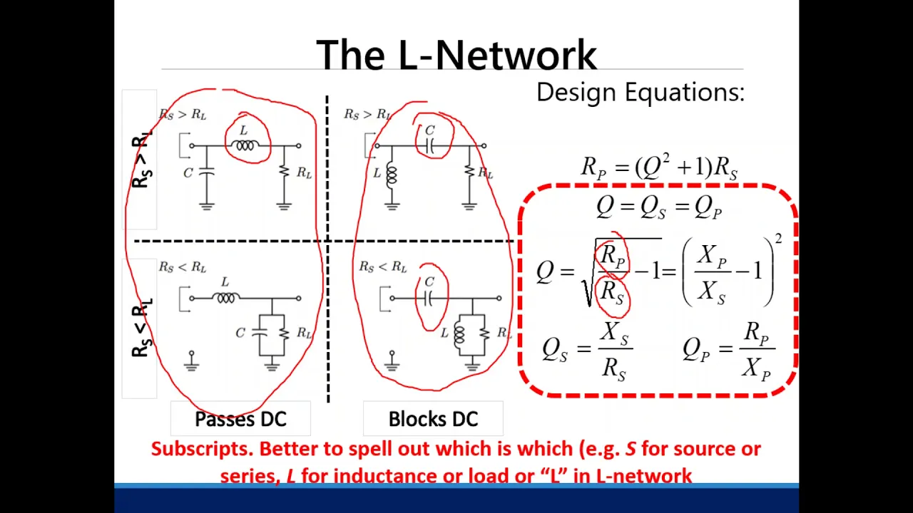
so this is kind of giving you a little bit of a hint that if i continue this circle all the way around that tells me that any impedance lying on that line is going to have the same 2.3 to 1 swr that's kind of interesting and we'll use that a little bit later on here so again let's talk about swr now on transmission lines okay so again i've got a complex impedance here and as i mentioned just on the previous slide if we just draw a circle that crosses that line centered at the center of the chart what we're saying is that the vswr and the return loss the magnitude of the return loss and the swr are the same for any impedance anywhere along that line so there's effectively an infinite number of infinite combination of complex impedances that will result in the same swr so that's kind of an interesting thing so as you can imagine as that circle were tighter and smaller around the center that swr would be smaller you get to the point where you're right at the center okay and and your swr is one to one so the larger that circle again the further you are away from the center the higher the swr is so why do we care about that well this interesting thing happens here is that rotating when you add or subtract transmission line length between your antenna and your transmitter you're effectively rotating around this curve on the smith chart if you add feed line length between your you know your antenna let's say you had you know 30 feet of coax and you added another 10 feet as you add that coax the complex impedance looking into that coax will rotate in a clockwise direction around this constant swr circle if we shorten the coax we rotate the other way now ideally you rotate and stay on this curve now if there's loss in the transmission line then you wind up getting kind of a spiral as you add more and more coax you're getting more and more loss instead of following the circle you're going to kind of follow a spiral and ultimately wind all the way up at the center if you had a really long piece of losses but let's let's assume lossless transmission line adding and removing transmission line will just literally rotate you around this constant swr circle so what's that also telling you is that ideally adding or removing feed line does not change your swr and you might say well i know if i change my coax length my swr does change well that can that will happen when the coax itself is part of the antenna system so for example if the shield of the coax is part of your counterpoi system either intentionally or not intentionally then you're going to then you're going to change the feed point impedance of the antenna by adding or subtracting coax which is also going to affect things but in those situations where your coax is not a radiating part of your antenna ideally you're not changing swr by adding a removing feed line you might also say well i've got i've got an automatic antenna tuner in my rig and you know it doesn't like tuning on 75 meters but if i add five feet of coax it does tune it fine so it must change the swr right it's going from one swr that it doesn't like and it's going to a different swr that it can tune to the reality is it's not changing the swr it's just changing the particular complex impedance that's being presented and that your tuner might have a hard time matching an impedance that's here but might not have a hard time matching an impedance that's here but it's still the same swr okay so all these interesting little facts kind of come out when you start studying transmission lines and feed line lengths so what's interesting also is that one complete trip around this circle is essentially a half wavelength of transmission line length so what that kind of implies is is that if i have if i have a transmission line length between my antenna and um and my transmitter and it's exactly a half wavelength long what that means is the impedance looking into the transmission line length is going to be exactly equal to the impedance of the antenna feed point if it's not half wavelength long then the impedance looking into the coax isn't going to be the same as the impedance looking into the antenna itself although the swr will be the same so every time you go a half a wavelength you repeat the impedance so again that's that's that's one of the magic things with a half wavelength line but now what's interesting is halfway around the like is a quarter wavelength line and there's a lot of magic things that happen with a quarter wavelength line you'll hear you know quarter wavelength trans uh tuning stubs and things like that but what they have quarter wavelength line does is an open will be transformed into a short and a short will be transformed into an open okay so if i took if i put a little t in my coax line and i put it and i just hung a piece of coax off at the end of that t and i left the end of it open right didn't put anything on the other end of it at a frequency where that's a quarter wavelength long that would look like a dead short so it could be a pretty effective notch filter for that one for that one frequency so uh so really so pretty interesting you could actually have an open-ended transmission line that at a particular frequency will look like a short now this again repeats every quarter wavelength right so at one quarter wavelength it'll do this transformation another quarter wavelength you're back to repeating the impedance go a quarter wavelength around again and it goes back and inverts quarter wavelength around again and repeat and it repeats so the odd quarter wavelengths do this transformation the even quarter wavelengths do the repeats of the impedance so again all this is kind of showing on the smith chart there's kind of cool stuff so let's take a look at uh adding coax lengths in an actual practical measured thing i did within my nano vna so i got the same 20 meter antenna that i'm measuring with just gradually increasing the line length by certain amounts so here's my starting point that's kind of the plot that i showed you earlier so there's my complex impedance okay going from 13.7 megahertz up to 14.7 megahertz here's my swr curve so now remember what we said that we're just going to rotate around the center of the curve but rotate around on that that constant swr circle so what that means is that essentially every point on this curve is going to rotate it around its own circle around the center okay so this this point right here in the center that's going to rotate it on its own little circle right here the 13.7 point is going to rotate on a much bigger circle okay so so there's my starting point so here i added about three feet of coax so you can see my curve the whole thing kind of rotated around now it didn't go it did maintain its shape perfectly and the reason for that is because the length of the coax is effectively longer at 14.7 megahertz than it is at 13.7 megahertz right because at 14 14.7 that's a shorter wavelength so the length of the coax in wavelengths or fractional wavelengths is actually longer for the higher frequencies so that this point actually rotates around a little bit further than this point rotates around so not only is this whole curve rotating around clockwise around the center it's also kind of compressing a little bit okay as it goes around so that was adding three feet of coax there's another three feet of coax i took that curve and rotated it around a little bit more and another three feet of coax and rotate it around a little bit more now you'll notice the the curve is a little bit tighter here now it's like closing up a little bit more than it is over here and again that's because this nine feet of coax that i added is more of a fractional wavelength at 14.7 megahertz and it is at 13.7 but now here's the really important thing no change in swr look at my swr curve in all these cases there's my white swr curve with the minimum swr right here there's my swr curve there's the swr curve and there it is again it didn't change in changing and adding these different lengths and coax and the minimum swr is still at the same point and every one of those right because all these points just rotated around the center but pretty cool stuff something maybe i didn't realize is happening but this is what's going on when you're adding and subtracting coaxially you're changing the complex impedance but you're not changing the swr so what can we do with that so well what's one thing that's interesting is you can say well okay i know i've measured at my antenna or actually at my transmit end here here the shack this is the complex impedance i measured here now if i know the transmission line length between my transmitter and my antenna i can essentially measure the impedance at the transmit end and then figure out what the impedance is at the antenna okay so if we expand on this portion of the smith chart we can actually see that these outer axes like with the numbers out here are calibrated in wavelength towards the generator and wavelengths towards the load so remember how i said half a wavelength around is is a complete trip around so we're starting at zero and rotating up so there's point zero four there we go all the way around here's point four nine and guess what point five would be right there right and same thing coming around the other way there's my point zero four i go all the way around here's 0.48 0.49 and back so we're using those those scales when we rotate around so again i can measure the impedance at the transmitter and predict the impedance at the antenna so if i measured the impedance here i would rotate now at the transmit end i would rotate towards the load right by if i know the length of my line i can say okay my line is this long okay i'll just go by the right the right fractional uh wavelengths and say that's the impedance at the antenna itself and that might be handy because you know ideally we want the antenna itself to represent a nice resin to match the transmission wine impedance so we really want our matching circuit to be at the tre at the antenna end so but you can do that by measuring the impedance at the transmit end and if you know the line length you'll know what the impedance is at the transmit i think excuse me at the antenna okay so you can use that to maybe design a matching network so i want to talk a little bit about resonance and minimum swr because it's another myth that i want to kind of dispel here a little bit and as i mentioned kind of towards the beginning that resonance only the definition of resonance is that only means that the reactance of the complex impedance is zero okay it doesn't mean that's where your minimum swr is so i i didn't i didn't cut crop this picture right but this is actually the center of the smith chart you can kind of see these these circles and the constant resistance circles kind of going through there so there's my center of the smith chart okay so this point right here is my 50 ohm point that i'm kind of pointing to so if we take a look at that you know i got the marker you know at the point that's closest to that but now how many resonant frequencies are there on this curve right there's one right there and there's another one right there so i actually have two they say now if you want to think about it this antenna and its coax is resonant at two frequencies but neither of those are where the minimum swr is so the minimum swr does not always occur and oftentimes does not occur at the resonant point so we're all kind of so accustomed to saying hey let me tune my antenna so it's resonant and what we're really doing is tuning for a minimum swr not necessarily tuning for resonance right resonance doesn't mean minimum swr and they don't always coincide uh but they're they're usually they're usually reasonably close but they don't have to be because generally the closer and closer you get to your ideal you know 50 ohm resistive point the smaller the reactive component is going to be but it doesn't it isn't always going to be zero so how do we set up the nano vna to measure an antenna or an antenna system meaning the antenna and its feed line normally what that means is you're going to select the traces you want to look at and you might just choose to put the swr trace up right this like the white trace right here and not have the others i like using the swr trace because this is what you know we kind of grew up you know using for the last 40 or 50 years i also like putting up the log magnitude on the not a via nano vna they just call it log mag but it's really the log magnitude measured on channel 0 which is the s11 we could do s parameters a whole nother talk on that but it's really just the reflection coefficient so it's the log magnitude of the reflection coefficient so that's the yellow trace that's this one right here and i like having that up there because the swr curve can tend to be a little bit shallow okay whereas the log magnitude is a bit more sensitive because of the way it's computed that more clearly shows you right where that minimum point is okay it's a lot easier to see that minimum point is here and sometimes the swr is a little bit shallow so the the log magnitude of uh of s11 could give you sometimes a clearer point of where your minimum swr is and then i like also having the smith chart up here as well okay and for reasons that we'll see in a moment so you would set up the nano vna to turn on the traces that you want in this case they're all measurements on channel zero and they're just different one is complex impedance one's log mag of s11 and one is swr and i turn the fourth trace off so turn your traces on configure them the way you want then you go and you set your stimulus range and i mentioned you don't want to set the stimulus range too wide because the the any vna has got a limited number of points that it will do kind of out of the box most of the nano dnas were 101 points later firmware updates brought them higher than that i've got one that'll do 401 points there's some out there that'll do 601 points and that's actually the actual points where the calibration is done okay and in between those it has to do essentially an approximation or an interpolation between those calibrated points so you don't really want to calibrate over the entire hf band if you're trying to measure an antenna on one particular band you certainly can but then it might make sense to have and these nano vnas allow you to save multiple calibration slots so you might have one that's set up wide band and then one then others that are set up just for the bands that you're you're typically interested in so you set your traces set your stimulus range run your calibration okay again the calibration sets up the measurement plane uh i've got some videos on this and this again is another topic we can go into but we'll just talk about you just it's just a good idea to calibrate where your transmitter connects so you're gonna so the nanovna is going to see what you're at what your transmitter sees and then go make your measurements so i'm going to play a video here this is about six minutes long and it's a it's a most of video number 314 it's going to show you those steps that i just outlined and also then show you how you can use the nano vna when you're adjusting your manual tuner so uh sit back and and watch this and then we'll come back and talk some more you can see that the yellow trace is already set up to be the log mag of the reflection coefficient so we'll leave that the green trace is already in smith chart so we'll leave that one alone so we'll reconfigure the blue trace to be swr and then get rid of the purple trace so we bring up the menu go to display go to trace and let's first just get rid of purple trace by touching on it touching how to get into to get rid of it and then we'll select trace number one the inverse text tells us we're selected we'll go back and then tell it to be on channel zero which is the reflection reflection channel or the s11 channel and now we just have to go back in one more time to the format and hit swr next let's set up the frequency range we want to test so bring our menu back up and go back and back again and go to stimulus in our case i want to measure the 40 meter amateur radio band from 7 megahertz to 7.3 so i touch on the start frequency and i dial in 7 m for megahertz that will set up the start frequency and then we'll go back in and select stop frequency 7.3 megahertz and now we've set up the stimulus range that we want to test the next thing we want to do is run the calibration so we go bring the menu back up go back and hit cal and go to reset to reset the existing calibration we can see that those calibration indicators have gone away over here and then we hit calibrate and since we're only doing a reflection measurement on channel 0 we only have to do an open short and load so we start off by putting the open on the port and touching open and next we put a short on the port and touch short and then we replace the short with a 50 ohm load on the port and touch load once we've done all three standards we can hit done and then choose to save it to a memory location i'm going to choose just to save it to location one so now we hook up the antenna with the antenna hooked up we can see our swr plot over the 40 meter band we can see the log magnitude of the reflection coefficient and we can see the smith chart and we can use the jog wheel to move our cursor or marker to make measurements at various frequencies across the range or we even have some marker functions to search for a min or a max so for example if i touch on on marker number one that activates trace number one and i can go into the marker function and do a search and search for a minimum and that will put the marker right at the minimum and i can see that's at 7.216 megahertz now of course that's all we need to do if all we want to do is to sweep the antenna but if we want to retune it for example we can leave these displays up and actually watch the reaction as we adjust the tuning of the antenna so let's say for example i want to retune to be closer to the middle of the cw portion of the band instead of in the phone portion where it is now so we can actually just watch the reaction on the vna as i tune the controls on my antenna tuner and this is where i find it handy to have the smith chart shown on the vna because you can actually see how the controls on the antenna tuner are going to twist and roll the trace on the smith chart and it gives you a little bit better intuitive feel about which way to tune the various controls now the first thing i'm going to do is move my marker down to oh somewhere in the cw portion of the band maybe around 7.07 7.06 7.05 something in the neighborhood so to give me an idea that's the the point that i want to now try to optimize with the tuner all right we'll start by moving some of the dials around here let's take a look at how the various curves move around we can see as i turn my inductor up i can see the smith charts kind of turning around in this direction and we can actually see i'm bringing my marker on the smith point smith chart closer and closer to the center of the smith chart so i'm getting kind of close but it's still kind of missing the mark a little bit so we're probably going to optimize the capacitor here as well so if we tweak on that a little bit i can see i'm deepening the null there on the reflection coefficient and i'm getting pretty close so you can see with just a little more fine-tuning on the controls of the tuner i've got myself pretty darn good at my desired point right there swr is about 1.02 i'm sitting right at the center of the smith chart so so hopefully that was kind of an it's kind of a fun way to play with the nano vna and to uh and to really see what your tuner is actually doing to the complex impedance so um yeah it's just kind of a neat thing to do so also kind of get used to what the smith chart showing you and relate them to swr and that type of thing so the last part of the the chat here i was going to talk about designing an l network impedance matching network and a little bit of extra credit here for those that might be interested i know this might uh is a bit more of an advanced topic but just just i think it's helpful to kind of go through and see this is how the smith chart was used before we really had you know kind of automated tools to you know do some of our calculations for us to design matching networks we can kind of do it somewhat graphically so let's run through that process so an impedance matching network like an l network or a pi network is really just adding series and parallel inductors and capacitors to essentially move the impedance around to make it look like our desired impedance in this case our system impedance or 50 ohms okay so an l network is the simplest network to use and its topology uh which topology to use is going to depend a bit on what the load impedance is and this is kind of yin yang diagrams if you will that will kind of indicate what the most appropriate um configuration of the l network is now i've got another network tuner here i've got it you know my 10 tech 238 tuner is an l network tuner and it can switch between two different networks depending on whether the impedance is high or low but if your impedance is somewhere in this kind of clear area here then this network will work we take our here's my complex impedance a shunt capacitor followed by a series inductor we can match anything in this area down to our down to where we want it to be and conversely you know this one here is a shunt inductor and a series capacitor and then these th these two um again a little bit different um show the other networks here as well and then there's also this other subset here where you got two capacitors or two inductors you can actually make a nail network with two of those and there's a limited set of complex impedances that they can match and you'll find oftentimes that more than one topology will work okay so if my complex impedance was somewhere over here i could use this topology or this topology right because both of those are in that white area so why would i choose one of the other um it might be due to you know what components you have on hand right the value of the inductor and capacitor used in this network will be different than this one and you might have you know one on hand and not the other for example or you might want your matching network to you know be a high pass or low pass filter right so in this case this this matching network is more of a a low pass filter it will filter away a high order harmonic so that might actually be a good thing okay because it's going to filter harmonics away if you want your matching network to be a high pass filter you might choose this okay so there's a number of considerations that you might choose to pick which topology you know because in many cases you have a choice of at least two okay so what happens when we add you know these inductors capacitors what happens to the impedance how do we move it around right because the idea is we've got an impedance that's non-ideal it's not resonant it's not at 50 ohms but we want to move it to here how do we get there okay but we talked about adding elements in series in parallel so when we add these components we're going to move the impedance around on the chart okay adding series inductors or series capacitors meaning a an inductor or capacitor in series with your load is going to move us along the constant resistance circles like this so if we add a series inductor it moves us kind of this way clockwise along those constant resistance circles and and uh by an amount that you can kind of compute here so here i went from a inductive reactance you know normalized reactants of 0.8 to 1.4 which means i moved a normalized reactance value of 0.6 ohms inductive okay multiply that by 50 that tells us how much inductive reactance i need to add right going adding a series capacitor moves us in the other direction along the constant resistance circles okay clockwise and counterclockwise okay and we could do the same thing figure out how far we went so but that's all for adding series components if we're adding components in parallel uh we usually will do that computation by talking about admittance right admittance is essentially one over impedance okay because when we add things in series like we add resistors in series we just we just add them up right r1 plus r2 plus r3 gives us our total right but when we have we're adding elements in parallel we add the inverses of them so we say 1 over r1 plus 1 over r2 plus 1 over r3 equals 1 over r total and then we can invert that to get the total resistance so those one over you know resistance or one over complex impedance we call that admittance okay so it's handy to deal with things in admittance when we're adding the parallel elements so the admittance is really just one over the complex impedance and just considering each component itself if we just have pure resistance okay then one over resistance is something we call conductance and if we just had a pure reactance okay at a pure x one over that would be the susceptance so we call that b but the reality is is that if we have a complex impedance it's not as simple as just inverting each element there is a it's a bit more complex than that okay so converting an impedance in to admittance is really easy on a smith chart mathematically it's tricky when you have a complex impedance on a smith chart it's really easy okay so on a smith chart there's my complex impedance there so if i want to convert that to admittance i draw my my constant swr circle centered around the center i bisect that circle with a straight line that goes through the center and touches at the other end and then that value is the complex uh admittance so in this case i've got a 1 plus j 1.1 right here and when i invert that then the admittance is 0.45 minus j 0.5 siemens okay what's up we talked about the smith chart and the uh impedance curves both the resist resistance and reactance curves there is also a way of designing a smith chart that will show admittance curves and it really is nothing more than rotating this chart by 180 degrees okay it's just inverting the chart by rotating it around uh so that's kind of what we did you know on the previous slide right we went halfway around that circle so it's the same kind of a thing and what i've been showing here all along but wasn't necessarily so obvious is that this is actually a combination chart all those red lines red circles and the red arcs represent the resistance and induct or reactants but if you look carefully there's also a set of blue lines in here and they're they're centered the other way those blue lines are all the admittance lines the conductance and susceptance circles are conductance circles and susceptance arcs okay constant conductance constants acceptance so as you can imagine uh when we talked about adding elements and seriously walk we went walked our way up and down the constant resistance circles when we're adding elements in parallel we're going to walk up and down the constant conductance circles okay so adding a parallel inductor is walking up uh the constant conductance circle that way again we're on the blue lines now and adding a parallel capacitor we're going down the other way so again this is really easy to do with the combo smith chart because uh those blue lines are there and then we're reading the blue numbers over here to figure out how far we went so how do we remember which way we go with all these things so here's my my corny little quick tip on how to do this so when we're adding inductors whether they're in series or in parallel we're elevating through the real axis okay so if we're adding a series inductor we're elevated or going up through and we're kind of going this direction you know where we cross the real axis okay and then we're adding a parallel inductance we're again elevating you know through on the constant conductance circles and even more corny when we adding capacitors we see crashing down through uh the center axis so a series index a series capacitor is going along the constant resistance circles a parallel capacitor is going along the constant [Music] conductance circles so now you can kind of see that by adding series and parallel inductors capacitance we can walk away from any impedance on the chart walk our way down to and zigzag our way to the center of the chart to create an impedance match that's actually how it works so let's go take a look at the process so if i'm going to design an l network the first thing i'll do is usually draw you know and highlight my cut my r equal 1 and my g equal 1 circles they're going to help me here in a moment this is where i want to get to right here in the center maybe this is where my starting point is knowing my starting point i can go to my little yin yang diagrams and figure out what topology i want to use so in this case it's it's first a series inductor followed by a parallel capacitor so what we're going to do is add our series inductor from this point and keep adding that until i hit my constant conductance circle and depending on where i was i might do that until i i'm gonna i'll try and hit one of these circles right so i'm gonna hit that constant conducted circle okay now now i've got the inductance value that i added and then i'm gonna add a in this case a shunt capacitor so i'm going down on my constant conductance circles here until i reach the center and again reading off the the uh these scales on the blue axis here i can figure out how much capacitance i added and there's my my l and c so let's do a practical example of it okay just by computing this so here's my practical example let's say i'm operating at 432.1 megahertz i measured my complex impedance of 75 ohms minus with a of reactants of 60 ohms and normalize that plot that on the smith chart okay that's where i am so that's where my complex of beans is this is where i want to get to i'll look at my yin-yang and say okay i'm going to use this topology so i'm going to start off with you know going from my load i'm going to start with a shunt inductor and then a series capacitor so let's go to the next step so i'll first kind of again highlight my r equal 1 circle and i'm going to now i'm gonna i'm adding a shunt inductor so that means i'm going along my constant conductance circles okay like this blue line right here i'm going to follow that all the way up until i hit my my r equal one circle now i gotta go take a look at how far i moved so if we look down here if we follow this down that's between point three and point four so it's about a point three two and so that move from there to zero and then from there up to this point here which is on the 0.5 line so i basically moved a normalized susceptance of 0.82 siemens right so that's how far i moved so that's how far i went i can invert that to get to the complex the normalized inductance of 1.22 i multiply by 50. so this tells me that i want to add 61 ohms of inductive reactants and knowing my operating frequency i can then take that's the reactants i want 61 ohms divided by 2 pi times that 431 432.1 megahertz it tells me my inductor is 22.5 nano henders okay so that got me up to this point step three now is i want to add my series capacitor that's going to rotate me down along my my constant resistance circle to the center so i rotate that down i can see that i i added 1.2 ohms or 1.2 normalized ohms of capacitive reactance multiply that by 50. again that gave me 60 ohms of capacitive reactants and again knowing my operating frequency i can compute the capacitance value from that 6.14 peak of variance so now i've got my l in the matching network that took my complex impedance from my antenna and now transformed it to look like a 50 ohm resisted input impedance so that's how you design a an old matching network using smith charts i know it's a lot easier to plug numbers into a calculator and just get it or a simulator or something like that but this is the way it was done graphically before we had those tools available to us and it's just kind of cool to see how it all works so i've got a number of videos on my channel that are related to nano vnas in terms of the basics and things like that i've got number 312 is the basics of what a vna is what's a vna itself and then talks a bit more about the nano dna i've got a whole video dedicated to and talking about how how and why we do a bna user calibration another one 314 is the one that i kind of showed you is measuring an antenna observing that tuning process uh 316 uh how do we measure antenna coax length with the vna number 325 talks about the effect of adding transmission line length that's what the one where i got those pictures that i showed you where we added three feet at a time uh number 326 is how to measure the impedance of an unknown hunk of coax and then also it does another one 334 is showing how to tune a dupe like a repeater duplexer with a nano dna so but it's just a couple of examples of vna videos that i've got available so in summary you know smith chart is a pretty highly useful tool for looking at swr looking at return loss you know doing transmission line impedance transformations understanding the effect of adding or subtracting transmission lines maybe designing matching networks and things like that and there's a whole lot more that you can actually do with it but this is just kind of what we touched on here today thanks again for watching this presentation i know the folks at the san fernando valley amateur radio club uh enjoyed it and i hope you did too thanks again as always for watching and we'll see you again next time
Up Next
5:51
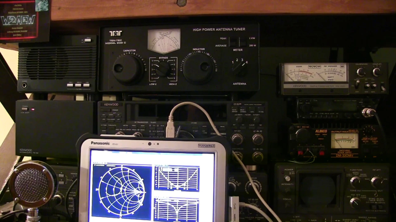
Visualizing Antenna Tuner Operation With a VNA and Smith Chart
@w2aew
53.9K views•2017-07-17

30:32
Ultrasonic Transducers: Resonant Frequency Measurement and Horn Design
@imajeenyus42
229.9K views•2017-02-22

54:16
Polymer Environmental Degradation: Mechanisms & Stabilization
@iit
1.8K views•2012-07-10

33:39
How a Student's Question Saved a NYC Skyscraper from Collapse
@veritasium
22.8M views•2025-04-26
Related Study Plans & Knowledge Roadmaps
Structured learning paths in Engineering
engineering
Building Acoustic Levitators: Physics & Arduino
01The Physics of Sound and Standing Waves
02Piezoelectric Transducers and H-Bridge Drivers
03Arduino Programming: Generating 40 kHz Signals
+ 2 more learning modules
14h5 modules
Explore Roadmap
engineering
Building Peltier Cloud Chambers: Particle Tracks
01Cosmic Rays & Cloud Chamber Physics
02Thermoelectric Cooling (TEC) Fundamentals
03Custom Liquid-Cooling Loop Design
+ 2 more learning modules
18h5 modules
Explore Roadmap
engineering
Yagi-Uda Antennas: Modeling, Build & VNA Test
01Introduction to RF and Antenna Fundamentals
02Yagi-Uda Antenna Design Principles
03Antenna Modeling and Simulation in 4NEC2
+ 2 more learning modules
18h5 modules
Explore Roadmap
engineering
ECG Monitor Design: Op-Amps, Filters & Noise
01Electronics & Breadboard Basics
02Op-Amps and Instrumentation Amplifiers
03Bioelectricity and ECG Fundamentals
+ 2 more learning modules
18h5 modules
Explore Roadmap