![Build Your Own End-Fed Half-Wave Antenna [A Complete Guide to EFHW]](https://i.ytimg.com/vi_webp/SBrc1DpMk_w/maxresdefault.webp)














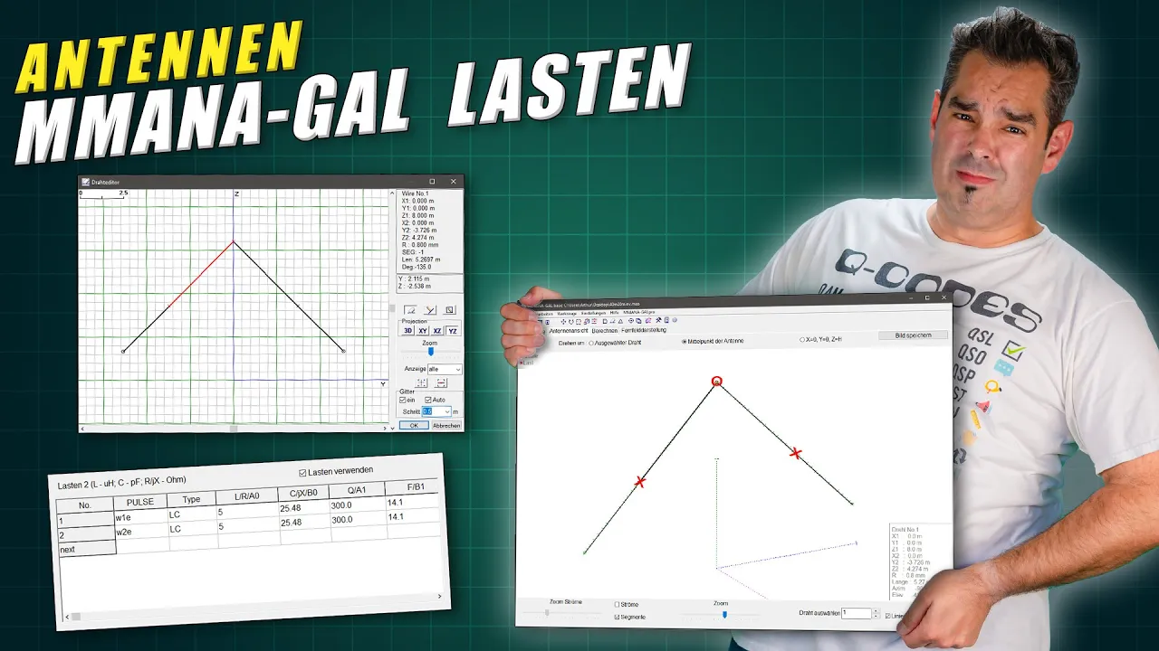




This video demonstrates how to simulate an End Fed Halfwave (EFHW) antenna using MMANA GAL software, showing the complete workflow from setting up geometry with X1/Y1/Z1 and X2/Y2/Z2 coordinates to calculating SWR and radiation patterns, with optimization techniques to improve impedance matching and visualization of far-field plots including 3D rendering and elevation analysis for DX communication.
EFHW Antenna Radiation Pattern Simulation in MMANA-GAL
Added:Fundamental principles of End-Fed Half-Wave (EFHW) antennas, including their resonant behavior and high feedpoint impedance.
Basic concepts of radio frequency (RF) engineering, such as Standing Wave Ratio (SWR), impedance matching, and the function of UNUN transformers (e.g., 49:1).
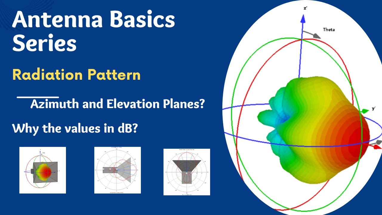
Understanding antenna radiation characteristics, including gain (dBi), elevation and azimuth patterns, polarization, and far-field distribution.
Familiarity with basic computer-aided design (CAD) concepts or the general layout of antenna modeling software.
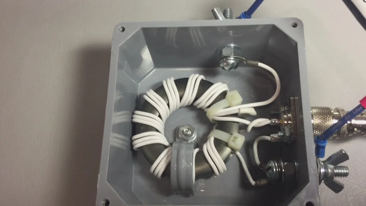
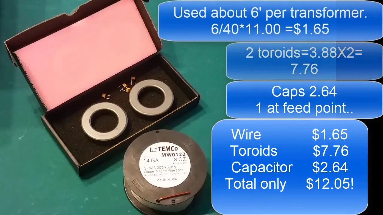
Physical implementation of EFHW antennas, including constructing 49:1 or 64:1 impedance matching networks (UNUNs) using toroidal cores.
Analyzing the impact of real-world environmental factors, such as ground conductivity, dielectric constants, and varying antenna heights on radiation patterns.
Advanced MMANA-GAL techniques, including multi-band optimization, geometric wire editing for complex configurations (like L or Inverted-V shapes), and utilizing the NEC-2 engine for more accurate ground modeling.
Field testing and validation of simulated antennas using diagnostic tools like Vector Network Analyzers (VNAs) or antenna analyzers to correlate empirical data with simulated plots.
12.1K views261likes23:34Original Release: 2023-05-22
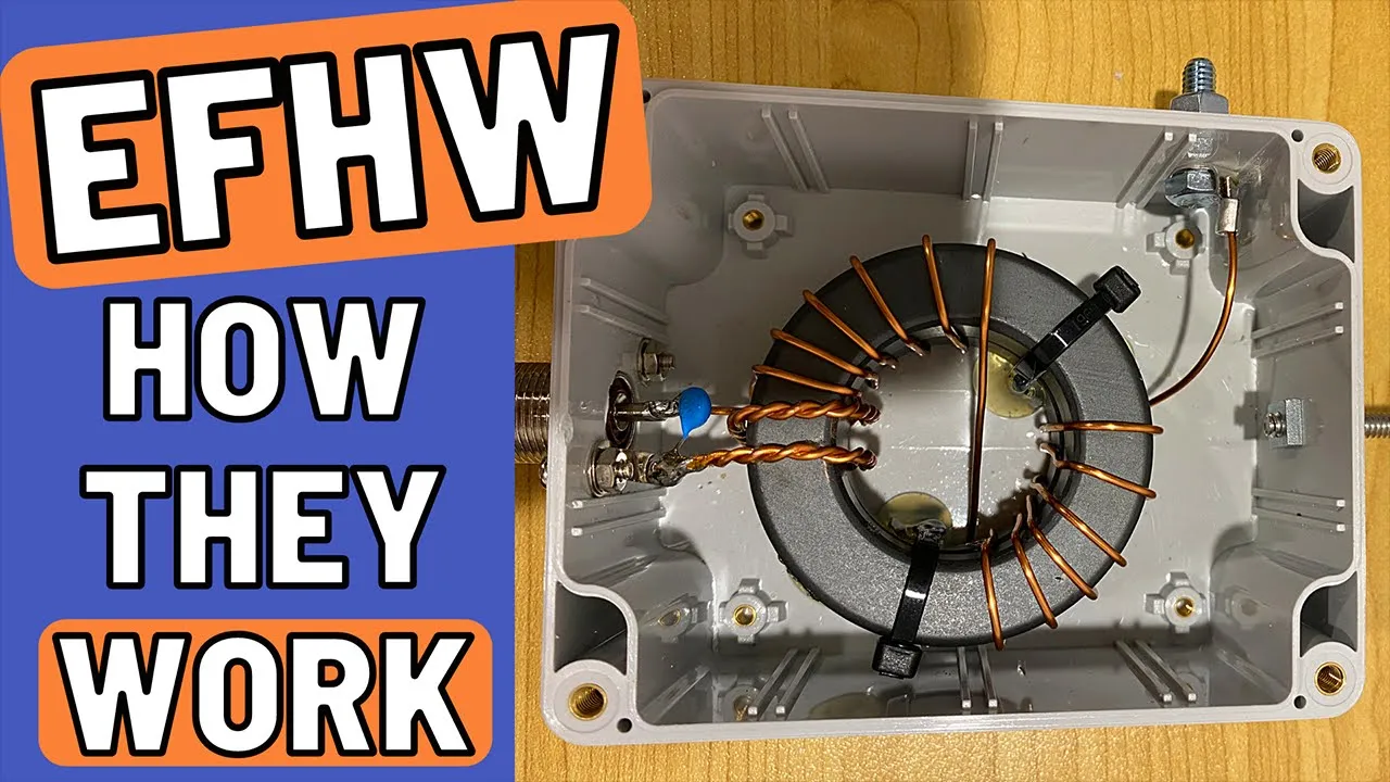
we are going to model an end fed half wave antenna using manigal so first we start the manigal application here the program launches and a few words about the program itself we are using right now manigal basic you can contribute to the effort of the programmers by upgrading and paying for manigal pro however for this exercise we're just going to leave the freely available manigal basic on the screen note that we have the menu bar up here we have some quick icon access tools up here and then we have our four tabs geometry view calculate and for far field plots in Geometry is where we specify the geometry with X1 y1z1 which we're going to leave at the origin X2 y2z2 essentially in three space the beginning and end points for our antenna in the view we're going to go ahead and see our antenna we can hold down the mouse and move it sideways hold down the shift key move it up and down so we can actually see our design a little bit better and calculate this is where the main action of the program takes place we're going to click on the start button when we're done with our modeling to actually start the program to run the actual calculations and notice here that we have the ground definition box right here we're now going to select free space perfect we're going to go with real and the ground setup button here allows us to modify a dielectric constant or a conductivity and and also when you're dealing with vertical antennas of course radials are important so you check this box right here we're not going to do that in our case since we're not going to be working with a vertical also notice if the ground that you're trying to model is say for example close to salt water or hard Rocky denser terrain or swampy wet ground you're going to have to look up the dielectric constant and the conductivity for those scenarios in our case we'll leave the defaults we say okay the material that we're going to use is going to be copper wire you have some options here our nfit half wave is going to be a copper wire and the height we're going to leave it at one meter one meter being about three feet so three feet off the ground in passing we notice that all of these entries are going to be in meters so we need to convert from feet to meters so let's get started first we're going to go ahead and say the title for our project is efhw or n fed half wave antenna and then for the frequency we are going to select 21050 you can enter the value here but we're selecting the CW portion of the 15 meter band next what we do is we highlight the X1 cell and we say enter and we are given x y z of zero and X2 y2z2 of 0. so here we're going to go ahead and put in some values what values well let's look at our geometry our field geometry or what we expect to have is an antenna that is going to have a 49 to 1 Transformer here a little pigtail which is actually going to be this counterpoise or really it's going to be the sheath of the coax cable this is a coax cable go into our radio the radio would be down here this is the 67 feet long wire that I'm going to perch up on a tree and 67 feet comes down to 33 and a half in height and 58.02 feet in in displacement in the X Direction you're just using Pythagoras's Theorem to come up with these numbers again manigal uses meters that's the M over here in these values so I converted 33 and a half feet to 10.218 meters similarly 58.02 feet comes out to be 17.68 meters so let's go ahead and enter these values and see where we are we leave the origin X1 y1 Z1 at zero and X2 we're going to be putting in here that one was 17.68 meters enter Y2 are going to be flat against the X Z uh plane so we're not going to put any Y2 displacement and on this one we're going to put 10.218 because that was the height or the Z1 parameter let's make sure 17.68 is our X and 10.218 srz 17.68 10.218 so all is good now what we're going to do is we're going to go to view to see if this actually works the way we expect it well if we look over here we see that we have an antenna in the X Z plane there we go there he is that's the X axis right there and the z-axis so if we move it this way you see that the antenna is with y equals to zero in other words it's flat against the X Z plane back there great by the way here you can zoom although there's not going to be too much of interest there but you can actually zoom in here and you can hold the shift key and move the antenna sideways up or down so there we are the shift key and the mouse key of course okay so are we done well let's go ahead and put our feed Point down here and for that we right click and we say add the source at the beginning of the wire and notice here now that managal has added a little circle a red circle right here if we look at the legend the red circle means that's the source that's where we're driving our antenna with and now if we go back to Geometry tab there's something interesting that has happened if you notice now the program took that source that we just added interactively and added this thing which is the source on wire one at the beginning a voltage of 10.0 volts are going to be used to simulate or drive this antenna simulation great so now are we ready to calculate well one thing to note we could hit start right here and the program would start calculating 21.05 we double check that we're on the right frequency that we want the simulation to run we notice in here that says swr50 so he's going to assume that your feed Point has got 50 ohms of resistance that's not what we actually have what we actually have is a little bit different so we want to go ahead and say setup and here we want to change the what he's going to use for an SWR of one to 2450 that's actually when you use a 49 to 1 Transformer that's actually going to be your SWR normally you corrected that with the 49 to 1 Transformer great so now let's try our luck we click Start and we end up with a very high value 574 for SWR and our resistance is not good 360 ohms so let's see if we can do something to simulate a little pigtail notice here we didn't put a little pigtail or the little coax going over to our radio let's see if we can model it again how do we add an antenna element on manager easy highlight the X1 box and click enter great we leave the origin at zero zero zero that's the beginning of this element and this one the X2 we're going to change it to minus two so what is this minus 2 well that's minus 2 meters or say about six feet of coax going from the 49 to 1 Transformer back to our radio let's see what the view looks like well the view looks like actually what we expected it to we can go ahead and see the little pigtail or counterpoise as it's accurately called there so let's go and try to calculate here click on start and now we're doing a lot better not resistance wise but SWR wise we're doing a lot better here so 2.97 now remember we have not added any loads we're not modeling any loads right here if we were we would get according to the legend a little X showing up at the little feed point we're not doing that so what we want to do and notice over here there's nothing on the load section what we want to do now is use a very interesting functionality of the program to say optimization notice right now we have not gone into far field plots yet let's hold off on going into far field plots and see if we can get that SWR a little bit better so click on an optimization is interesting because here managal in a very interactive way tells us hey what do you want to have optimized and what do I need to tweak to get that optimization for you these slider bars go from least important to most important on the right so least important on the left we don't want that to be least important SWR we want to be very important the match not least important we want it most important current and we don't care IX or JX as the double E's call it and we leave that at zero elevation yeah front to back ratio again we'll leave everything pretty much least important except for SWR and match and what do we want to tweak well we're going to tweak the length of the wire so let's first go ahead and see if we can tweak the length of our wire for the counter poise so for this we click on type and we say there's a bunch of parameters you can optimize here and one of them is wire okay so here we do wire and we're going to do wire one the X parameter I'm sorry the my the the uh that'll be wire two actually so we want to change that to wire two which is our counter Poise and then we're going to go ahead and say optimize click on that one X2 remember X2 was actually at a minus two meters so that's exactly what he's going to do so it's going to go to minus two kilometers over to two kilometers let's go ahead and put that one to zero and then over here I don't know let's put that one to minus 50. we're not going to be doing any more than that step 0.01 that should be okay so let's go ahead and start and he is optimizing right now he's actually done optimizing in 1.8 seconds do we want to save the optimization lock yeah and now what he's done is he's gone ahead and given us actually a little bit of a worse value there so let's go to geometry and he's changed it over here to minus 3.83 so you know again with optimization you have to be careful that the mathematical solution is actually making sense and in this case not so much so let's go ahead and say that we want to change that to well let's leave that one there but let's optimize also wire one in other words we select wire and we're going to do to both parameters of of wire one what are those parameters if you remember we had X2 which was I believe it was uh 17.68 well there it is 17.68 meters and the other one is the height or Z2 remember that was a 10.218 so we're going to tell it hey not only can you optimize this pigtail but you're also going to be able to optimize the length of our wires and again we're going to go here 50.
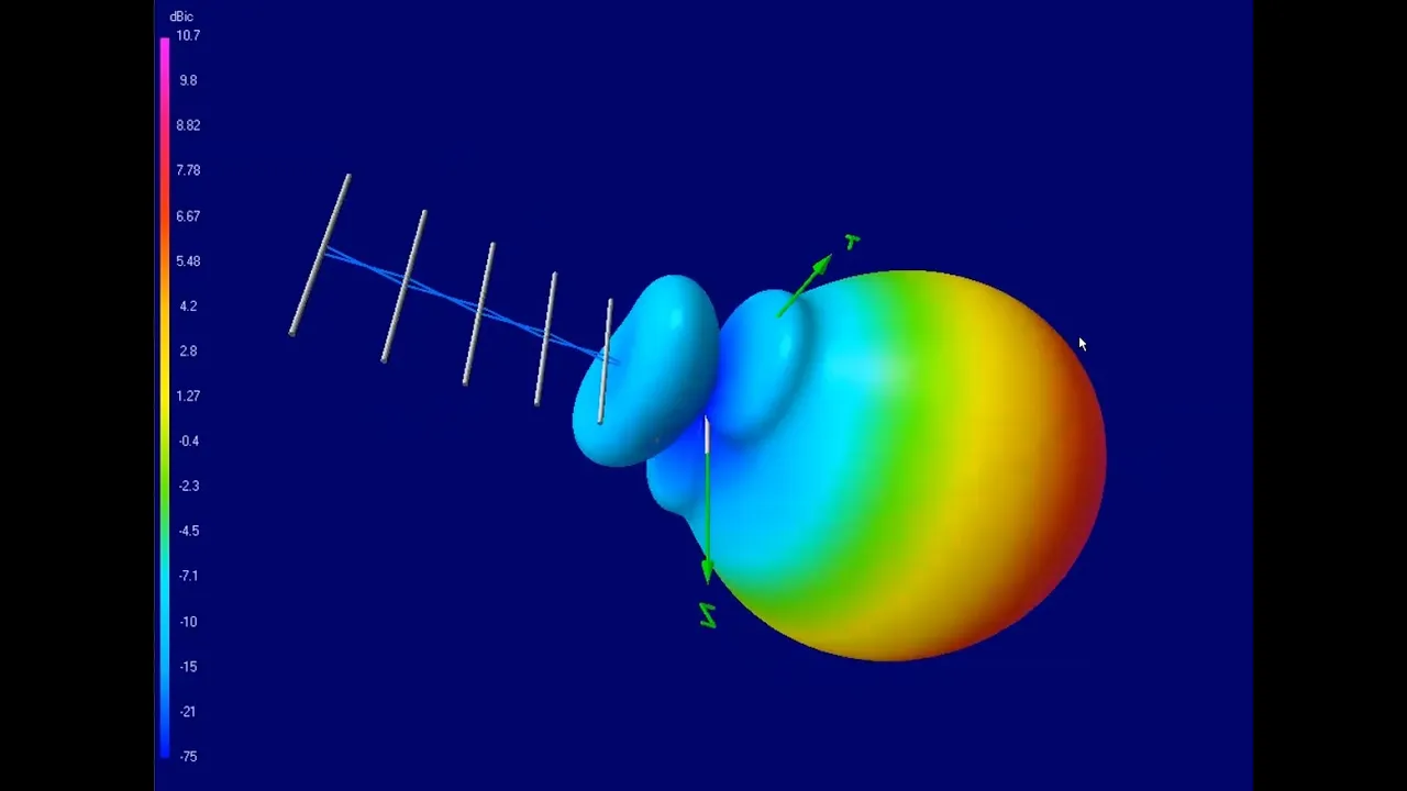
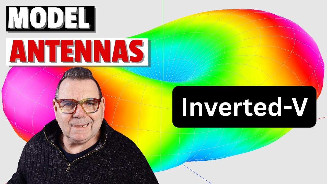
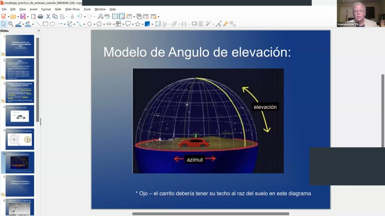
then we have to hit return or enter and we're not going to go anything like that so zero 250. great so now let's say start and now he's able to optimize a few more parameters and we notice now that the SWR has gotten a lot better do we want to save the optimization log no and the resistance is quite high but is it it's really going to be 24.50 so it's trying to get it very close to 24.50 here so 2443 is actually a good value we don't want this in other words to be 50 ohms we want it to be what the 49 to 1 Transformer is going to be able to transform down so 1.05 sounds pretty good but what has this actually done well let's run right down it's essentially run right now it's actually run in optimization but nothing has been written to to the pro to the file to this session so let's click on start and he runs it with those same parameters gives us the same results but now he's actually written this information so let's go back to our geometry tab see what he's changed and if you notice here he's changed a few things this used to be 17 points 68 I believe and this used to be 10.218 so the program has optimized this length so he's telling us to make sure these lines are a little bit longer so that's great he's given us an idea hey don't don't cut your wire exactly to 67 feet you might want to cut it longer so that you can go ahead and uh and and make make sure that it resonates well now this is according to the theory and well how many feet is that going to be for the length of the wire again that's the X displacement and the Z displacement so we have to use Pythagoras to go ahead and come up with the actual length of the wire which we can do but right now let's continue with outputs of our program again he has moved the length of our little pigtail installers hey you probably want to make a longer pigtail okay great how long well 3.8 meters that's going on about 12 feet of of coax that may not be realizable but we can you know keep that in the back of our mind he's asking us to the program is asking us to make a longer pigtail and to calculate we already did this so now if we go to the far field thoughts this is interesting that he's giving us now is giving us an asymusal plot over here and a cross-section plot or elevation plot over here what is this telling us well think of this as a methyl as a bird flying right over the antenna that's the that's the antenna High Point right there and I'm sorry that's the origin that's the that's where the antenna starts and then the bird keeps on going this way this is the positive X Direction here and so on so and this over here is like like you took a chainsaw to it to this and you came up with the cross sectional or the elevation profile why is this called the elevation profile because if you think about it would you really care for DX it's a low elevation otherwise one of these lobes should be quite low so this is telling you that you're going to have a bit of good DX going in this direction and a little bit of good DX going in this direction oh hang on what about these guys well these are going to be Cloud burners what do you mean well they're going pretty much straight up into the sky so you're going to have an envis you know remember what that is from our test that was near vertical incidence scattering or something to that effect so essentially that's too high so that the wave is going to go the electro electromagnetic wave that Fermi radio is going to go straight up and pretty close to straight down this one's going to go way out before it bounces off of the ionosphere so that's all great but you know we like to think more in terms of 3D well manigal can allow that there's 3D fast Fourier over here and he's given us a little 3D plot what step yeah take the default okay and now he's giving us a pattern that we might be able to understand a little bit better so there right there there's a light blue wire right there that's the antenna So the antenna is actually going from the origin which is your feed point out here to the tree and then you see that pattern so it's telling us hey you're going to have a lot of the energy going here there but most of it's going to be going in this direction however the one thing that we're interested in is this right here so that is actually going to be a good DX pattern and then this one over here these two are going to be also good DX patterns this is the cloud burning part of the antenna so that's another feature to image the radiation pattern in 3D using pretty much software that's easy to use and it's free managal basic now there's one other thing to point before we call it quits and that's the elevation remember we talked about an elevation of how many degrees say about five to eight degrees is pretty good for DX as a matter of fact uh Callum McCormick the DX Commander when he models his antennas using managal he uses an elevation of five degrees for DX so we can actually set that five degree elevation to see what the pattern would be at five degrees so you click on elevation and you click five and enter so now the patterns changed a little bit well yeah because now he's essentially taking the cross section at the five degree Mark over here this one over here is still pretty much a cut across like a chainsaw tilt to it but this one right here now is telling you that lobe right there remember the closer to the edge there the more gain you've got and uh it's actually quite good so if we go actually in using the mouse we can see over here now that an anatomous angle of say minus 180 which is you know going in the minus X Direction you will have a gain of minus 1.8 DBI now the interesting thing here is that the gain is relative so this program really gives you an idea of where your most your highest gain is where your lobes are where your highest gain is over there and so on so you can compare this lobe to this slope for sure but don't get so hung up on the actual magnitude of DBI remember when you see advertisements with antenna sales people they might say well my antenna's got a a gain of 7 DB well great but you know they never tell you at what elevation what's the actual profile so we're getting a lot of information here and this right here also gives you that elevation that it's saying that it's a this angle right here you're probably going to get the best elevator the best gain and on this side over here that's nine degrees so that's a good DX part of the antenna there is going to be giving you somewhat good gain but not as good as this side over here so that is a quick introduction to managal the other thing that we can do without too much effort is this is what it looks like at 15 meters what if we were to change this to other frequencies say for example we want might want to use this at 18.08 you know at the at the 17 meter so we go ahead and do that it gives us a 35 to 1 SWR there so that's not so good so don't expect it to work according to the program at 17 meters what about 20 meters we change that to the CW portion of 20 meters click Start 1.45 the program is saying hey you might actually get this to work pretty well according to Theory at in the 20 meter CW portion well let's continue playing this game what about 40 meters CW click on start 3.2 now it could be worse you might be able to actually get a tuner and actually correct for that and then what about at the uh 80 meter band well in that case yeah that's not going to work so the antenna is not going to work so good there and to complete this we can actually go over to some of the frequencies to see how they would work according to the model it's not so good for that that band either and at 10 meters actually is going to go to what according to the math it's going to look pretty well there so we're starting to get an idea okay for this completeness sake at six meters and okay not not too bad so it's telling us that it's going to have multiple frequencies in which this is actually going to work fairly well having the 15 meter band which is the one that we might be interested in working the best so that is a quick view of there are other buttons by the way the plots buttons also gives you some information this but this is a quick view of managal and essentially again how quickly it is to enter a geometry view visualize your geometry make sure it makes sense make sure that your geometry and xyz's is not messed up and then here you can also add your source calculate you can go ahead and click Start and get the this amazing program to go ahead and calculate and give you some some information and very importantly the optimization tab right here is the one where you tell it what you can vary given what you're really wanting to optimize for and that's the last thing you can find out the far field plots again remember these far field plots are going to look different than what we looked at earlier because we're in a different frequency range so remember depending on the frequency range your far field plots are going to look different so this is what we're seeing right here and another feature that we saw was the 3D fast Fourier over here for the 3D plot of our antenna just for Grants we can look at this one take the default step and you start seeing how these parameters can actually look how these radiation patterns can actually look pretty involved and again that light blue line right there is our antenna you can picture the tree being over here sort of like what our sketch had up here and the origin were the 49 to 1 Transformer is being at the at the at the origin of this plot and a little pigtail going out that way in the minus X Direction so hopefully this was useful managal it's a good tool and you you'd be surprised about what you can simulate with it with a few clicks and how the program suggests things to try out hopefully that was helpful
Up Next

12:31
Gamma Match Antenna Tuning Explained for Ham Radio
@madeinfoxtrap5539
63K views•2023-01-16

12:54
Triumph of Orthodoxy Icon: Byzantine Art & History Explained
@BenCallan
2.1K views•2024-08-06

9:49
FastAPI vs Flask vs Django: Choosing the Right Python Web Framework
@TechWithTim
302.5K views•2024-05-26

1:42
Game of Thrones Opening Credits: A Cinematic Analysis
@gameofthrones
46.3M views•2011-04-18
Related Study Plans & Knowledge Roadmaps
Structured learning paths in General & Interdisciplinary Studies
general-studies
Elevator Engineering: History, Physics & Cities
01From Hoists to Safety Brakes: The Dawn of Vertical Lift
02Hydraulic vs. Traction: The Engineering Physics of Elevators
03Modern Speed, Safety, and Algorithms
+ 2 more learning modules
12h5 modules
Explore Roadmap
general-studies
Rubber: Material Science, History & Geopolitics
01Origins of Natural Rubber & Mesoamerican History
02The Chemistry of Natural Rubber & Vulcanization
03The Geopolitics of the Rubber Boom & Colonization
+ 2 more learning modules
12h5 modules
Explore Roadmap
general-studies
Containerization: Evolution, Logistics & Trade
01Ancient Trade & Bulk Cargo: Amphorae to Barrels
02The Industrial Revolution & Cardboard Packaging
03The Containerization Revolution: Malcom McLean
+ 2 more learning modules
12h5 modules
Explore Roadmap
general-studies
Textile Tech: Evolution, Labor & Global Impact
01Pre-Industrial Textiles: Handloom & Cottage Industry
02Mechanization: The Spinning Jenny to the Power Loom
03The Factory System & Global Labor Transformation
+ 2 more learning modules
10h5 modules
Explore Roadmap