A MEMS vibrating structure gyroscope measures angular velocity using a silicon ring structure with eight asymmetric legs, where driving elements oscillate the ring at a known frequency and sensing elements detect Coriolis forces acting on the structure during rotation, enabling precise angular rate detection through the cosine 2 theta mode resonance vibration.
MEMS Vibrating Structure Gyroscope: Inside the CRS03-01T Angular Rate Sensor.
Added:Deep Dive
The physics of the Coriolis Effect, specifically how rotation induces a virtual force on a moving or vibrating body.

What is the Coriolis Effect?
290.6K
The Coriolis effect is a fictitious force that appears to deflect moving objects when observed from a rotating reference frame, such as Earth's surface; it causes large-scale phenomena like hurricanes to rotate counterclockwise in the Northern Hemisphere and clockwise in the Southern Hemisphere, but it is too weak to affect small objects like toilet water, which are instead influenced by local factors like bowl imperfections and floor levelness.
Click to watch →

The Ingenious Evolution of Gyroscope Technology
424.6K
During the 1980s, another theoretical method for measuring rotational rate was being developed into a practical mechanism called a vibrating structure gyroscope or Coriolis vibratory gyroscope. This type of gyroscope uses the principle of vibration to measure rotational rate. The key principle behind its operation is the Coriolis effect, which affects a vibrating object when its support structure rotates—as this rotation occurs, the vibrating object tends to keep vibrating in its original plane, resulting in a Coriolis force exerted on the support. By measuring this force, the rate of rotation can be determined.
Click to watch →

How Stuff Works??: Gyroscopes Explained | Physics & MEMS Technology
150.1K
The Coriolis force or Coriolis effect is a fundamental physics principle that enables measurement of rotation or angular velocity. When a body of mass m moves in the x-direction with velocity Vx and experiences angular velocity ω in the y-direction, it experiences a Coriolis force. This force is a vector quantity that is perpendicular to both the velocity in the x-direction and the angular velocity in the y-direction. The magnitude of the Coriolis force is proportional to the mass of the body, its velocity, and the angular velocity. The direction can be determined using the right-hand rule.
Click to watch →

Best Demonstration of Coriolis Effect on YouTube
587K
The Coriolis force is a fictitious force that appears to deflect moving objects to the right in a counterclockwise rotating system; this can be demonstrated using a rotating parabolic dish where marbles follow straight paths in an inertial reference frame but curved cycloid trajectories in a non-inertial rotating reference frame.
Click to watch →

The Coriolis Effect
612.4K
The Coriolis effect is an apparent deflection of moving objects that occurs when observed from a rotating frame of reference, such as Earth's rotation; objects moving in straight lines appear to curve because the observer is rotating, which explains phenomena like hurricane rotation patterns (counterclockwise in the Northern Hemisphere, clockwise in the Southern Hemisphere) and affects long-range projectiles, though it does NOT cause water to spiral down bathtubs or toilets.
Click to watch →
Deep Dive
Fundamental concepts of Micro-Electro-Mechanical Systems (MEMS), including silicon micro-machining and scale effects.

MEMS and NEMS devices
9.1K
MEMS (Micro Electromechanical Systems) are devices operating at 1-200 micrometer scales that convert electrical to mechanical energy and vice versa. They integrate micro sensors, actuators, microelectronics, and mechanical structures on silicon substrates through deposition, patterning, and etching processes. Key advantages include enhanced speed, reduced complexity, lower power consumption, smaller form factors, and superior system integration. The large surface-to-volume ratio at micro scales makes surface effects dominant, enabling unique mechanical behaviors through thin coatings. Applications span automotive (airbag accelerometers, tire pressure sensors), medical (blood pressure monitors), and consumer electronics (inkjet printers).
Click to watch →

Distinguished Research Lecture 117–Professor Victor M. Bright
468
MEMS combines micro-scale electrical and mechanical components fabricated on silicon wafers, ranging from 100 micrometers to a few millimeters. Richard Feynman's 1959 vision predicted that miniaturization would enable revolutionary technologies, later realized when IBM arranged individual atoms in 1990. The key insight is that as objects shrink, surface-to-volume ratio increases dramatically, making surface phenomena like tension and adhesion dominant over bulk properties. This explains why water striders walk on water and geckos climb glass—smaller scales amplify surface effects. MEMS leverages existing semiconductor fabrication infrastructure, enabling high reliability, low costs, and consistent performance through mass production.
Click to watch →

MEMS Micromachining Overview 9/9/2014
35.1K
MEMS encompasses three primary micromachining approaches: surface micromachining using CMOS-compatible processes, bulk micromachining for three-dimensional structures, and LIGA for high-aspect-ratio fabrication. MEMS operates at the micron scale (~1 micron minimum), significantly larger than integrated circuits (~20 nm), because mechanical components require sufficient physical dimensions to function. Surface micromachining follows a layer-by-layer sequence: deposit sacrificial layer (silicon dioxide), pattern and etch holes using photolithography, deposit structural layer (polycrystalline silicon) conformally, pattern structural layer, then remove sacrificial layer to release movable parts. Photoresist serves as a light-sensitive mask protecting underlying material during etching. The sacrificial layer analogy compares to keystone bridge scaffolding—temporary support removed after structural components are properly formed.
Click to watch →

Mod 03 Lec 11
584
MEMS (Micro Electro Mechanical Systems) integrates electronic and mechanical components at the micro-scale. Micro machining adapts traditional machining processes (turning, milling, laser) for micrometer-scale fabrication. Two main types exist: bulk micro machining creates structures inside substrates via selective etching, while surface micro machining builds structures on top using film deposition and selective etching. Micro scale is defined as 10^-6 meters, enabling batch processing of thousands of identical elements simultaneously on single wafers for devices like sensors and integrated circuits.
Click to watch →

This "Old-Fashioned" Tech Is Means To Perfecting Autonomous-AI | Dr. Diego Emilio Serrano | Ep53
272
MEMS combines microelectronics fabrication techniques with mechanical device construction, using semiconductor industry batch processing to create miniaturized devices with mechanical degrees of freedom. Starting with silicon wafers, layers are deposited and etched to produce movable structures. Key applications include accelerometers (detecting acceleration through capacitance changes) and gyroscopes (measuring angular velocity via Coriolis-induced displacement). MEMS serves as the critical interface between computing systems and the physical world, enabling modern technologies from smartphones to automotive safety systems and drones. Design requires multi-physics understanding encompassing mechanical, electrical, thermal, and fluidic domains.
Click to watch →
Deep Dive
Basic principles of mechanical vibration, resonance, and acoustic/vibrational modes in ring-shaped structures.
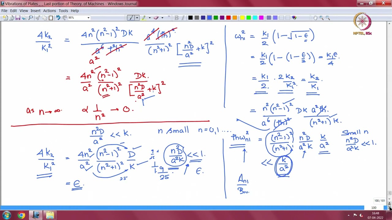
Lec 31 Insights into vibrations of rings
175
Circular rings exhibit distinct vibration modes characterized by natural frequencies and mode shapes: (1) Rigid body modes with zero natural frequency include pure torsional rotation (n=0, first set) and pure translation (n=1, first set), where the ring moves without oscillation; (2) The breathing mode (n=0, second set) shows pure radial oscillation where the ring expands and contracts uniformly; (3) Higher modes (n≥1, second set) exhibit coupled radial and torsional motion where the ring simultaneously oscillates radially and in-plane, with particles accumulating on one side during compression and on the opposite side during tension. The frequency expressions depend on mode number n, ring radius a, material density ρ, thickness h, and stiffness parameters k and s.
Click to watch →

Finite Element Examples. Lecture 4.
1.1K
Acoustic modes become excited when structural vibrations couple with them. If structural vibration occurs in areas where the acoustic mode has high pressure amplitudes (such as the footwell), coupling is strong and the mode will be easily excited. Conversely, if vibration occurs in areas with low pressure amplitudes (such as the roof center), coupling is poor and excitation is unlikely.
Click to watch →

Prof. Jim Woodhouse: Introduction to the basic physics of stringed musical instruments Part 2
682
This lecture introduces the fundamental principles of structural vibration using accessible examples. A vibration mode is a specific way a structure can vibrate, characterized by a unique resonant frequency and mode shape. Structures like drums and metal rulers can vibrate in many different ways simultaneously. In circular membranes, vibration modes are classified by nodal lines (regions of zero displacement): circular nodal lines create concentric stationary rings, while nodal diameters are straight lines through the center where no movement occurs. The total vibration response of any structure can be completely determined by adding up contributions from all its vibration modes—a principle called superposition. When a force is applied at a specific location, it excites different amounts of each mode (changing their amplitudes), but the mode shapes and resonant frequencies remain unchanged. This explains why hitting a drum at different positions produces different sounds. These principles apply universally to all vibrating structures including musical instruments.
Click to watch →

Vibration due ri Bearings ,Looseness and Resonance
17.9K
Mode shape is the deflected shape of a structure when a particular critical frequency is excited. When passing through the first critical, the center of rotation is at maximum deflection (anti-node). When passing through the second critical, the center point is at least deflection (node). When passing through the third critical, nodes exist at each end with two additional nodes about one-third away from the ends. Characteristics of resonance include: high vibration amplitude at specific frequencies (4-20 times higher than other directions), directional nature, existence during particular operational conditions (specific speeds or loads), lack of response to balancing, broken machine structure or welds, and 180-degree phase shift through resonant frequency.
Click to watch →
![[FEA1]-Speicherverfahren - Teil 1](https://i.ytimg.com/vi/DHKsi55mdgw/hqdefault.jpg)
[FEA1]-Speicherverfahren - Teil 1
495
Ring-shaped or cyclic structures present unique challenges for node numbering because they create unavoidable large index differences at the connection points between the start and end of the numbering sequence. Regardless of numbering strategy, these structures inherently produce significant bandwidth increases at the junctions. The resulting stiffness matrix will have full-width bands at these locations rather than the narrow banded structure seen in simply connected geometries, substantially increasing memory requirements.
Click to watch →
Deep Dive
The working principles of electromechanical transducers, particularly capacitive, piezoelectric, or electromagnetic sensing.
EE8403 - Transducers - Measurements & Instrumentation
356
Capacitive transduction is based on the capacitor principle with two conducting plates and a dielectric material. Capacitance changes with plate area, distance, or dielectric properties, and this change is calibrated to the measured quantity. Electromagnetic transduction is based on Faraday's law of electromagnetic induction, where changing magnetic flux through a conductor induces an electromotive force (EMF). In electromagnetic transducers, the physical quantity causes magnetic flux changes, inducing a voltage in a conductor. Self-generating electromagnetic transducers do not require external excitation, as the motion between magnet and electromagnet causes flux changes.
Click to watch →

Capacitive Transducer & Working Principle | Sensors and Transducers
1.8K
A capacitive transducer is a passive device that converts non-electrical physical quantities such as displacement, pressure, temperature, and liquid flow into electrical signals by measuring variations in capacitance, based on the principle that capacitance (C) equals the permittivity (ε) divided by the distance (d) between capacitor plates, and it offers high sensitivity, good frequency response, high input impedance, and requires minimal operating power.
Click to watch →

Capacitive Transducers - 1 | Sensors and Industrial Instrumentation | Lec 8 | GATE Instrumentation
6.8K
A capacitive transducer converts physical quantities into electrical signals by measuring changes in capacitance. The capacitance of a parallel plate capacitor is given by C = ε₀εᵣA/d, where ε₀ is permittivity of free space, εᵣ is relative permittivity, A is overlapping area, and d is distance between plates. Capacitance changes when any of these parameters are modified. The transducer works on the principle that capacitance is directly proportional to overlapping area and dielectric constant, and inversely proportional to distance between plates. By measuring these capacitance changes, the transducer can detect displacement, liquid level, or pressure.
Click to watch →
Lecture 16: Transducer Elements
5.1K
Two main types of transducers covered in this lecture are pneumatic transducers and electromechanical transducers. Pneumatic transducers convert displacement to pressure (such as the flapper nozzle system). Electromechanical transducers convert mechanical displacement or strain to electrical signals through various principles: Linear Variable Differential Transformer (LVDT) uses changing magnetic characteristics due to motion; resistance strain gauges use the principle that conductor resistance changes when stretched; capacitive transducers use changes in capacitance between plates due to motion; piezoelectric transducers generate electrical charge when crystalline materials like quartz are distorted by force.
Click to watch →

ME312 MI Lecture3 S6ME
241
Transducers can be classified based on the principle of transduction: resistance transducers, inductive transducers, capacitive transducers, thermocouples, piezoelectric transducers, optical transducers, and photoelectric transducers. In capacitive transduction, the measured quantity is converted into a change in capacitance by changing the distance between plates or the dielectric medium. In electromagnetic transduction, the measurement is converted to voltage induced in a conductor by changing magnetic flux. In inductive transduction, the measurement is converted into a change in self-inductance by displacing the coil core. In piezoelectric transduction, the measurement is converted into a change in electrostatic charge or voltage generated by a crystal when mechanically stressed. In resistance transduction, the resistance varies with the physical quantity, as in strain gauges.
Click to watch →
Prerequisite Knowledge
- Concept 01The physics of the Coriolis Effect, specifically how rotation induces a virtual force on a moving or vibrating body.
- Concept 02Fundamental concepts of Micro-Electro-Mechanical Systems (MEMS), including silicon micro-machining and scale effects.
- Concept 03Basic principles of mechanical vibration, resonance, and acoustic/vibrational modes in ring-shaped structures.
- Concept 04The working principles of electromechanical transducers, particularly capacitive, piezoelectric, or electromagnetic sensing.
Subsequent Learning
- Step 01Sensor Fusion algorithms (e.g., Kalman Filtering) to combine gyroscope and accelerometer data in Inertial Measurement Units (IMUs).
- Step 02Analysis of MEMS sensor errors, including bias instability, angle random walk (ARW), thermal drift, and Allan Variance calibration.
- Step 03Advanced MEMS resonator architectures, such as Disk Resonator Gyroscopes (DRGs) and micro-wineglass resonators for high-precision applications.
- Step 04The implementation of angular rate sensors in automotive safety systems, such as Electronic Stability Control (ESC) and rollover detection.
Device Intro
Core Structure
Transducer Roles
Operation Mode
Resonance Details
Visual Reference
Device Intro
0:00Playing Section
- 1
Examines a 1998 MEMS gyroscope.
- 2
Identifies it as a vibrating structure gyroscope.
Optical Gyroscopes and the Environmental Vulnerabilities of MEMS Vibrating Designs
While MEMS vibrating structure gyroscopes like the CRS03-01T are cost-effective and compact for consumer and standard automotive use, they face critical limitations compared to optical alternatives like Fiber Optic Gyroscopes (FOGs) and Ring Laser Gyroscopes (RLGs). Because MEMS gyroscopes rely on mechanical resonance and physical moving parts to measure the Coriolis effect, they are highly susceptible to mechanical shock, temperature fluctuations, and high-frequency acoustic vibrations. These environmental factors can induce resonant frequency interference, causing drift and measurement errors. In contrast, optical gyroscopes utilize the Sagnac effect, propagating light through closed paths. Lacking moving parts, optical sensors are immune to mechanical wear, vibration-induced drift, and acoustic interference, offering vastly superior bias stability and precision. For high-reliability, aerospace, or safety-critical autonomous driving applications, optical gyroscopes represent a crucial alternative that overcomes the physical and environmental boundaries of MEMS vibrating structures.
Deep Dive
Sensor Fusion algorithms (e.g., Kalman Filtering) to combine gyroscope and accelerometer data in Inertial Measurement Units (IMUs).
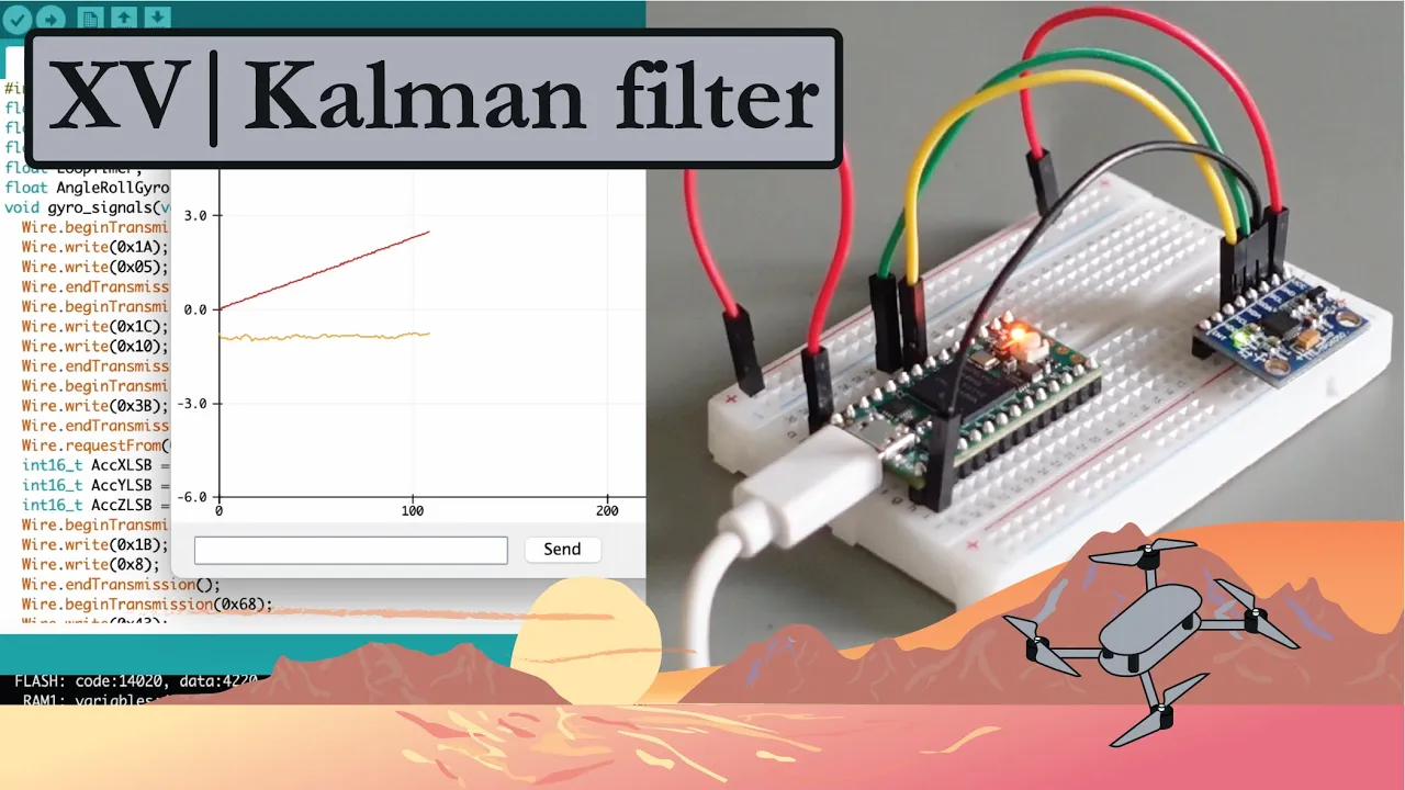
Kalman Filter for Gyroscope and Accelerometer Angle Fusion
228.7K
The Kalman filter is a mathematical algorithm that combines measurements from multiple sensors (gyroscope and accelerometer) to produce an optimal estimate of the true angle. It addresses the limitations of individual sensors by fusing their data in a statistically optimal way, reducing both drift errors from the gyroscope and vibration sensitivity from the accelerometer.
Click to watch →

Arduino 9 Axis, 9 Degree of Freedom Inertial Measurement IMU
34K
Sensor fusion combines complementary sensor strengths: accelerometers provide stable baseline values with no drift but are noisy and vibration-sensitive; gyroscopes provide clean changing signals with no vibration sensitivity but suffer from drift. By mathematically fusing these data streams, we achieve both stability and accuracy. This technique eliminates drift entirely while maintaining very low noise levels, enabling accurate roll and pitch measurement.
Click to watch →
GD4111 M10 - Gyroscope and Accelerometer
101
Sensor fusion combines gyroscope and accelerometer data for accurate orientation estimation. Gyroscopes provide accurate short-term orientation changes but suffer from drift over time due to integration errors. Accelerometers provide absolute orientation references based on gravity but are noisy and sensitive to external forces. The complementary filter applies high-pass filtering to gyroscope data (removing drift) and low-pass filtering to accelerometer data (removing noise). The filter coefficient alpha (typically 0.98) determines weight distribution. Alternative techniques include Kalman filters and Gaussian filters. Proper sensor fusion requires correct frame alignment and time synchronization between sensors.
Click to watch →

Kalman Filter for Beginners, Part 3- Attitude Estimation, Gyro, Accelerometer, Velocity MATLAB Demo
40.3K
Sensor fusion combines multiple sensor data sources to improve estimation accuracy. Gyroscopes provide continuous angular rate information but suffer from drift, while accelerometers can provide attitude estimates based on gravity direction when the body is not accelerating. Static attitude determination calculates pitch and roll from accelerometer measurements assuming zero inertial acceleration. By treating accelerometer-derived attitudes as measurements and integrating them with gyroscope data through a Kalman filter, the best estimate is obtained by leveraging the strengths of each sensor while mitigating their individual weaknesses.
Click to watch →

Intro to Inertial Measurement Units (IMU)
46.1K
IMUs are classified by sensor biases and drift characteristics, ranging from low-grade hobbyist units (accelerometer bias ~0.01g, gyroscope bias ~100°/hr) to high-end aerospace-grade units (accelerometer bias <0.00001g, gyroscope bias <0.1°/day). Since both gyroscopes and accelerometers measure orientation, sensor fusion combines multiple measurements to produce superior estimates. The Extended Kalman Filter fuses GPS, gyroscope, and accelerometer data to estimate positions, velocities, and orientations (state variables), compensating for individual sensor weaknesses. This multi-sensor approach leverages complementary strengths—gyroscopes excel at short-term rate measurement while accelerometers provide long-term stability—to achieve reliable drone state estimation.
Click to watch →
Deep Dive
Analysis of MEMS sensor errors, including bias instability, angle random walk (ARW), thermal drift, and Allan Variance calibration.
Gyro Noise Analysis Using Allan Deviation Plots
17.9K
This comprehensive workflow covers gyroscope noise analysis for aerospace systems: (1) Gyro fundamentals—angular rate sensors critical for inertial navigation in rockets; (2) Noise parameters—angle random walk (random fluctuations in °/√hr) and bias instability (drift rate in °/hr); (3) Allen variance analysis—a statistical method adapted from clock oscillator stability testing; (4) Data collection—logging stationary sensor data at 100 Hz for 6+ hours; (5) Plot generation—computing Allan deviation using Euler integration and plotting on log-log scales; (6) Parameter extraction—identifying Gaussian white noise (slope = -0.5), calculating angle random walk (×60 at τ=1s), and determining bias instability (min/0.664×3600). This enables accurate vehicle simulation and sensor selection for aerospace applications.
Click to watch →

Inside GNSS - High Performance Accelerometer Webinar - 07/08/20
537
Inertial navigation systems require distinguishing between day-to-day bias and short-term bias stability. Key requirements include: very low bias (critical for position accuracy), good long-term stability over years, accurate scale factor, low noise for fast tilt sensing, high vibration resistance, high bandwidth, low latency (<20μs jitter), mechanical stiffness for orthogonality, self-testing capability, and high MBD. Position error from accelerometer bias increases quadratically over time - 100μg bias causes ~1/300m error. The Schuler oscillation (84-minute period) limits error growth on Earth's gravitational sphere. Allan variance analysis characterizes sensor noise and bias instability, with MEMS now meeting QA2000 quartz accelerometer benchmarks.
Click to watch →

How to select the right IMU
3.6K
This comprehensive section covers the three fundamental parameters defining inertial sensor performance: scale factor (output-input relationship slope), bias (output at zero input), and noise (random variations). Measuring bias is challenging because stationary sensors detect Earth's rotation (gyros) or gravity (accelerometers)—requiring specific orientations for accurate measurement. Bias repeatability measures variation between power cycles, forming Gaussian distributions that factory calibration compensates for. Bias instability describes how bias varies during continuous operation, analyzed using Allan variance plots showing standard deviation versus averaging time. This reveals when noise filtering becomes ineffective—the minimum point representing inherent bias instability. Scale factor non-linearity describes deviations from ideal linear behavior, expressed as relative error (percentage or ppm)—a 0.1% non-linearity at 50 degrees/second produces 0.02 degrees/second error, creating 0.18 degrees of angle error during dynamic maneuvers. Velocity random walk and angular random walk characterize noise integration effects, measured similarly through Allan variance analysis. Two primary IMU technologies exist: MEMS sensors excel in size, weight, cost, and power for consumer applications but provide lower performance; Fiber Optic Gyroscopes deliver approximately 100 times better performance but require larger size, higher power, and greater cost. G-sensitivity affects mechanical gyros but not FOGs—no relationship exists between bias stability and G-sensitivity.
Click to watch →
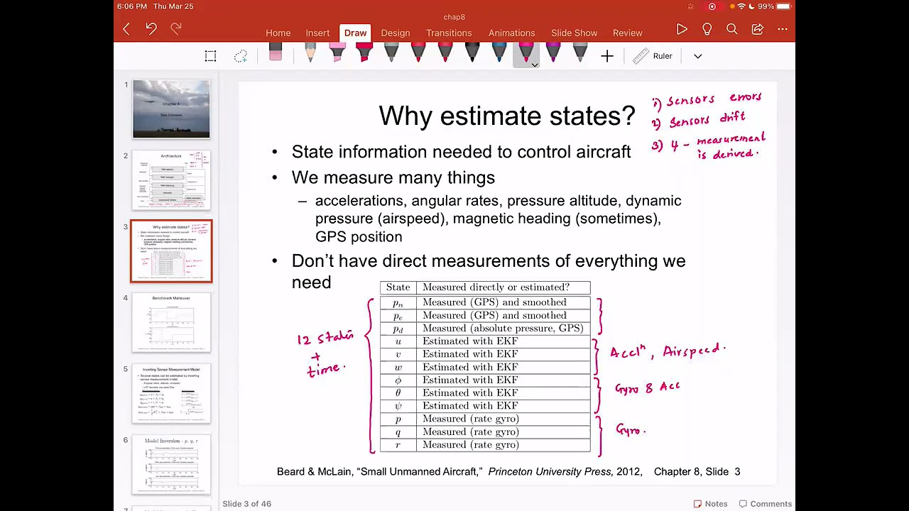
Robotics 2 lecture 22: 3.25.21
110
Gyroscopes have several error sources: (1) Startup bias - the gyroscope may start with a non-zero offset (e.g., 10, 0, or 120 degrees), (2) Random noise - stochastic variations in the output, and (3) Thermal drift - output changes with temperature. These errors cannot be completely eliminated by calibration but can be minimized. The complementary filter helps mitigate these errors by combining with accelerometer data.
Click to watch →
Visual-Inertial Sensor Calibration -- A Complete Tutorial and Discussion
20.4K
Accurate IMU noise characterization is essential for visual-inertial state estimation. The process involves: (1) Keeping the IMU stationary for extended periods (hours), (2) Computing Allan variance charts from the data, (3) Extracting white noise density and random walk coefficients from characteristic points. Recovered parameters should be inflated by factors of 5-10 times (white noise ×5, random walk ×10) to account for unmodeled noise sources. This inflation creates conservative estimates that prevent over-trusting the IMU. Continuous-time parameters should be used, with discrete-time equivalents derived from the IMU update rate.
Click to watch →
Deep Dive
Advanced MEMS resonator architectures, such as Disk Resonator Gyroscopes (DRGs) and micro-wineglass resonators for high-precision applications.
Encapsulated MEMS: What’s Good for the Resonator is Good for the Sensor, by Tom Kenny
2.4K
Conventional MEMS sensors use distributed perimeter anchors that make them vulnerable to package warpage and stress-induced drift. The breakthrough insight is that single-point anchoring eliminates this vulnerability entirely. For accelerometers, a single anchor connects a proof mass to differential resonators that measure acceleration through frequency shifts. For gyroscopes, the wineglass architecture uses a single central anchor with Coriolis coupling between in-plane modes. These designs achieve exceptional performance: sub-micro-g accelerometers and 0.135°/hr gyroscopes—comparable to or exceeding commercial products while maintaining stability. The lesson is that architecture choices fundamentally determine sensor stability.
Click to watch →

The Coming Revolution in MEMS Gyroscopes and MEMS Inertial Sensors
5.3K
This section presents the progression of gyroscope architectures from conventional to revolutionary designs. Traditional tuning fork gyroscopes use two tines in driving and sense modes. The quad mass gyroscope (QMG) achieves quality factors up to 2 million through balanced energy loss configurations, enabling ~0.09°/hr bias stability in 50-micron-thick devices. The hemispherical resonant gyroscope (HRG) achieves exceptional performance with quality factors approaching 30 million and sub-millidegree/hour stability. Microfabricated shell resonators use glassblowing techniques to create fused silica cups ~5mm diameter with 70-100 micron thickness, achieving ring-down times of ~500 seconds and bias stability approaching 0.01°/hr. These innovations demonstrate that non-rectangular shell structures outperform traditional rectangular MEMS designs.
Click to watch →

Inside GNSS - KVH Webinar - Inertial Goes Photonic, Explodes Gyro Technology - 05/28/20
376
The wine glass resonator gyro uses a wine glass-shaped resonator where rotation drives energy between vibration modes at 45 degrees, causing procession measured as applied rate. Silicon MEMS versions collapse this to 2D planar structures with more transducer mass per unit volume. ARFOG combines ring laser gyro and interferometric FOG architectures, using fiber coils as ring resonators for both multiple passes (high resolution) and long path length (sensitivity), enabling smaller coils. Key challenges include fibers for tighter bend radii and miniaturizing discrete components using photonic integrated circuits. Hybrid silicon photonics enables fabrication on low-loss waveguides with CMOS devices positioned over necked-down regions, pushing optical fields into active devices for phase manipulation.
Click to watch →

BEARS 2021: New Faculty - New Directions
426
Motion resistance (Rx) in MEMS resonators is proportional to frequency times gap to the fourth power, divided by DC bias voltage squared. This relationship means Rx scales almost linearly with frequency, which is problematic for high-frequency oscillators. However, because Rx is proportional to d^4, gap shrinking can compensate for the increase in Rx at higher frequencies. To lower motion resistance, researchers use composite resonators with multiple disks coupled mechanically by beams of different lengths (lambda/2 beams), which move unwanted modes to higher frequencies while multiplying the output current. Fabrication involves depositing isolation layers, polysilicon interconnect using oxide molding for thicker polysilicon, disc fabrication with oxide hard mask and polysilicon layer, thin high-temperature oxide for gap definition, electrode patterning, and HF release. A 199.2 MHz MEMS resonator with 20,000 Q and 36 nm gap achieved excellent phase noise performance with -173.3 dBc/Hz at 1 MHz offset.
Click to watch →

Farrokh Ayazi - "MEMS and Integrated Instruments: What does the future hold?"
486
Diamond resonators using nanocrystalline diamond with zinc oxide achieved 78 MHz operation. However, 3D wineglass resonators revealed that surface losses dominate dissipation in thin-film resonators, with Q independent of device dimensions. The surface loss mechanism depends on the ratio of shell thickness to lossy layer thickness, explaining why extremely thin films cannot achieve ultra-high Q factors. Monocrystalline silicon carbide offers superior MEMS properties: wide bandgap enabling high operating temperatures and radiation hardness, three times higher Young's modulus than silicon, higher thermal conductivity, and approximately 30 times lower intrinsic dissipation. Georgia Tech achieved record Q=20 million at 6 MHz using silicon carbide square lamina resonators with integrated acoustic crystals. Silicon carbide disc gyroscopes achieved 4.6 million Q with 10x better angle random walk than silicon counterparts.
Click to watch →
Deep Dive
The implementation of angular rate sensors in automotive safety systems, such as Electronic Stability Control (ESC) and rollover detection.
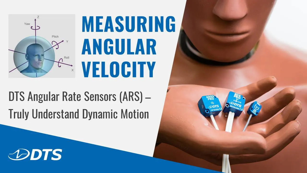
Angular Rate Sensors (ARS) - Truly Understand Dynamic Motion (44 min)
2.3K
Angular rate sensors must survive extreme shock and vibration environments (up to 150 Gs with superimposed vibration). The ARS Pro (2011-2013) addressed high-shock limitations in anthropomorphic test device calibrations, hard surface impacts, and military blast protection through improved linear acceleration fidelity, shunt test capability, reduced power consumption, and enhanced noise performance. Key features include: measurement ranges from 300 to 50,000+ dps, DC response for slow-position measurements, stable output across 4.9-14V excitation, 300-2000 Hz bandwidth meeting SAE/ISO standards, ISO 17025 calibration, and shunt check capability. Connection requires two excitation and two signal connections operating as a full bridge. Recommended setup uses 5V excitation, full bridge configuration, and 3000 ohm shunt resistance. Angular rate sensors are active devices with oscillating elements generating residual noise above 10,000 Hz, requiring filtering at 2000 Hz or below.
Click to watch →
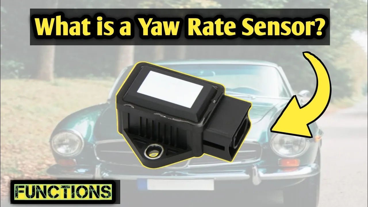
What is a Yaw Rate Sensor? Functions and Benefits
10.5K
A Yaw Rate Sensor is an electronic device that measures a vehicle's rotational movement around its vertical axis, detecting how much the vehicle is turning left or right; this sensor is essential for Electronic Stability Control (ESC) systems, which use its data along with steering angle and wheel speed sensors to detect loss of traction and prevent oversteer or understeer by selectively braking wheels and reducing engine power, and it also supports Roll Stability Control (RSC) for preventing rollovers in high-center-of-gravity vehicles like SUVs and trucks, while contributing to advanced driver assistance systems such as adaptive cruise control and lane keeping assist, and serving as a fundamental component in autonomous driving technologies by providing critical orientation data for maintaining vehicle stability and accurate positioning.
Click to watch →

How to Work..Yaw Rate Sensor
863
A yaw rate sensor detects the rotational movement of a vehicle during dynamic driving conditions such as passing through potholes or making turns, and sends this data to the Electronic Stability Control (ESC) system to properly apply brakes across all four wheels and to the Traction Control System (TCS) to maintain vehicle stability and prevent loss of control.
Click to watch →

EN | Bosch Angular-rate sensor SMG10x for rollover application
34.1K
Roll-over mitigation (ROM) systems utilize existing electronic stability control (ESC) sensors to reduce the risk of vehicle rollovers. ROM functions by detecting when a vehicle is subjected to extreme lateral tire forces, which can lead to loss of control and rollover. Upon detection of such conditions, the system initiates a sequence of corrective actions, starting with the braking of the outer front wheel. This targeted braking helps to counteract the lateral forces and stabilize the vehicle. The Bosch SMG10x angular-rate sensor is specifically designed for this application, providing precise measurements of vehicle rotation rates to enable accurate and timely intervention. The sensor integrates into the ESC platform, leveraging existing hardware to enhance safety without requiring additional major components. Its role is critical in ensuring rapid response to rollover-inducing conditions, contributing to overall vehicle dynamic safety. The system operates autonomously, relying on real-time sensor data to trigger corrective measures before a rollover occurs. This technology exemplifies how sensor precision and control logic work together to improve automotive safety in high-risk driving scenarios.
Click to watch →

차량동역학및제어 L#8. Rollover Prevention
1K
Rollover prevention systems operate through detection and activation phases. Detection requires conservative logic to avoid false positives that cause driver panic. The Rollover Index (ROI) combines roll angle and lateral acceleration to predict impending rollovers in real-time. Since direct roll angle measurement is impractical, lateral acceleration data provides approximation. Electronic Stability Control (ESC) integrates rollover prevention by reducing cornering or stabilizing yaw rate when ROI exceeds thresholds. The steady-state relationship AY = VX²/R connects vehicle speed, turning radius, and lateral acceleration, enabling predictive control strategies. ESP employs four key components: wheel speed sensors, yaw rate sensors, steering angle sensors, and a control unit processing sensor data. Active suspension systems enhance prevention by applying counteracting forces before rollover initiates, representing the state-of-the-art in vehicle safety engineering.
Click to watch →
Device Intro
Core Structure
Transducer Roles
Operation Mode
Resonance Details
Visual Reference
Device Intro
0:00- 1
Examines a 1998 MEMS gyroscope.
- 2
Identifies it as a vibrating structure gyroscope.
Optical Gyroscopes and the Environmental Vulnerabilities of MEMS Vibrating Designs
While MEMS vibrating structure gyroscopes like the CRS03-01T are cost-effective and compact for consumer and standard automotive use, they face critical limitations compared to optical alternatives like Fiber Optic Gyroscopes (FOGs) and Ring Laser Gyroscopes (RLGs). Because MEMS gyroscopes rely on mechanical resonance and physical moving parts to measure the Coriolis effect, they are highly susceptible to mechanical shock, temperature fluctuations, and high-frequency acoustic vibrations. These environmental factors can induce resonant frequency interference, causing drift and measurement errors. In contrast, optical gyroscopes utilize the Sagnac effect, propagating light through closed paths. Lacking moving parts, optical sensors are immune to mechanical wear, vibration-induced drift, and acoustic interference, offering vastly superior bias stability and precision. For high-reliability, aerospace, or safety-critical autonomous driving applications, optical gyroscopes represent a crucial alternative that overcomes the physical and environmental boundaries of MEMS vibrating structures.
The physics of the Coriolis Effect, specifically how rotation induces a virtual force on a moving or vibrating body.
Fundamental concepts of Micro-Electro-Mechanical Systems (MEMS), including silicon micro-machining and scale effects.
Basic principles of mechanical vibration, resonance, and acoustic/vibrational modes in ring-shaped structures.
The working principles of electromechanical transducers, particularly capacitive, piezoelectric, or electromagnetic sensing.
Sensor Fusion algorithms (e.g., Kalman Filtering) to combine gyroscope and accelerometer data in Inertial Measurement Units (IMUs).
Analysis of MEMS sensor errors, including bias instability, angle random walk (ARW), thermal drift, and Allan Variance calibration.
Advanced MEMS resonator architectures, such as Disk Resonator Gyroscopes (DRGs) and micro-wineglass resonators for high-precision applications.
The implementation of angular rate sensors in automotive safety systems, such as Electronic Stability Control (ESC) and rollover detection.
1.8M views57.7Klikes1:00@EvilmonkeyzDesignzOriginal Release: 2024-04-08
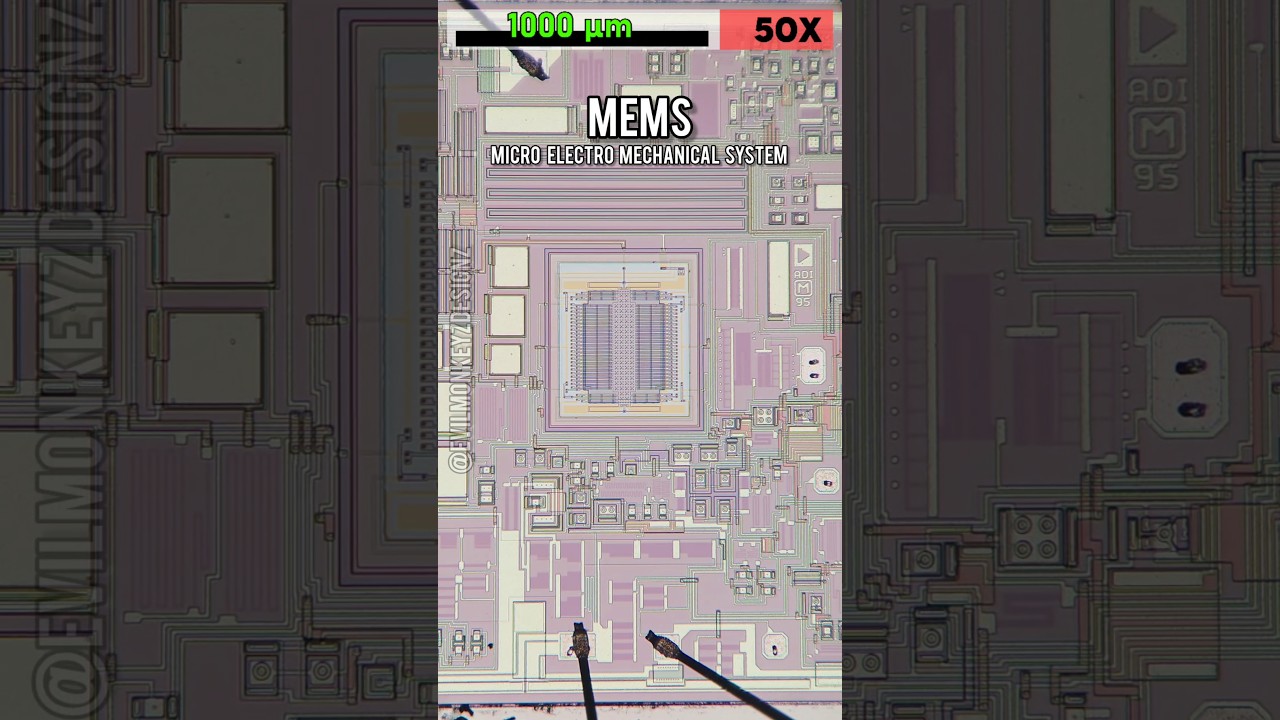
let's take a closer look at another mems device a gyroscope from 1998 specifically this is a vibrating structure gyroscope from Silicon sensing what's inside this device is actually quite surprising the actual mems part of this device is the Silicon ring structure that sits on top of a glass block which consists of a 6 mm diameter ring connected to eight asymmetric legs as far as I understand these eight legs are transducers and among them are driving and sensing elements the driving elements oscillate the structure at a known frequency while the sensing elements sense changes by forces acting on them mainly due to the coris effect the data sheet says it uses the cosine 2 Theta mode resonance vibration and there's also a main it involved somehow I haven't been able to remove the center structure but I found this picture online showing what it looks like underneath I also found a presentation with lots of interesting information about how the sensors have evolved over time we'll have to look at one of the newer ones next
Up Next
96:06
Linear Quadratic Regulator (LQR) Control Design Tutorial
@ChristopherLum
148.5K views•2018-12-03

30:32
Ultrasonic Transducers: Resonant Frequency Measurement and Horn Design
@imajeenyus42
229.9K views•2017-02-22
1:09
ADXL05 MEMS Accelerometer Teardown: 1996 Single-Axis IC Analysis
@EvilmonkeyzDesignz
3.7M views•2025-04-18

33:39
How a Student's Question Saved a NYC Skyscraper from Collapse
@veritasium
22.8M views•2025-04-26
Related Study Plans & Knowledge Roadmaps
Structured learning paths in Engineering
engineering
Building Acoustic Levitators: Physics & Arduino
01The Physics of Sound and Standing Waves
02Piezoelectric Transducers and H-Bridge Drivers
03Arduino Programming: Generating 40 kHz Signals
+ 2 more learning modules
14h5 modules
Explore Roadmap
engineering
Building Peltier Cloud Chambers: Particle Tracks
01Cosmic Rays & Cloud Chamber Physics
02Thermoelectric Cooling (TEC) Fundamentals
03Custom Liquid-Cooling Loop Design
+ 2 more learning modules
18h5 modules
Explore Roadmap
engineering
Yagi-Uda Antennas: Modeling, Build & VNA Test
01Introduction to RF and Antenna Fundamentals
02Yagi-Uda Antenna Design Principles
03Antenna Modeling and Simulation in 4NEC2
+ 2 more learning modules
18h5 modules
Explore Roadmap
engineering
ECG Monitor Design: Op-Amps, Filters & Noise
01Electronics & Breadboard Basics
02Op-Amps and Instrumentation Amplifiers
03Bioelectricity and ECG Fundamentals
+ 2 more learning modules
18h5 modules
Explore Roadmap