Rocker-Bogie Rover: Build, Stereo Vision & ROS
Learning Goal: Construct a six-wheeled rocker-bogie Mars rover chassis, derive and program its 6-wheel steering kinematics, and implement autonomous obstacle negotiation using stereo-vision depth mapping and 3D point cloud processing.
Prerequisites
- Mathematics: Basic vector calculus, coordinate transformations (homogeneous matrices), and trigonometry.
- Programming: Intermediate Python (with NumPy) and basic C++ (for Arduino/ESP32 firmware).
- Software Tools: Familiarity with Autodesk Fusion 360, OpenCV basics, and terminal-level Linux/ROS operations.
- Hardware Requirements: Access to a 3D printer, DC motors with encoders, steering servos, a PCA9685 PWM controller, an Arduino/ESP32, and two synchronized USB cameras or a custom stereo module.
Estimated Total Study Time
- 48 Hours (including hands-on design, electrical prototyping, and software configuration).
Module 1: Physics and Kinematics of Rocker-Bogie Suspension
Understand the mechanical advantages, passive suspension physics, and weight distribution of the six-wheeled rocker-bogie mechanism. This module establishes why this specific geometry is favored for planetary exploration, detailing how it maintains traction without springs.
Recommended Videos

Why this video is valuable: This documentary-style masterclass covers the engineering history and fundamental mechanics of Donald Bickler’s rocker-bogie suspension system designed for JPL. It details the exact mechanical problems the design solves—namely, maintaining constant, uniform wheel contact and equal load distribution over highly irregular obstacles without resorting to standard spring-shocks.

Why this video is valuable: This highly detailed 3D animation visualizes the physical components of the Perseverance Mars Rover. It provides an exceptional anatomical breakdown of how the differential bar, the rocker links, and the bogies pivot in relation to the main chassis frame.
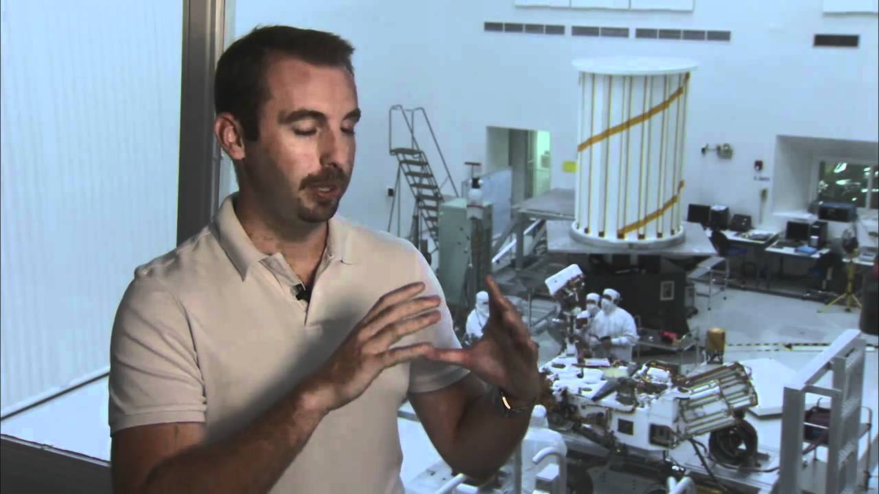
Why this video is valuable: A look at the physical prototyping of NASA JPL's Curiosity Rover. This video shows real-world tests of the system climbing over rocks larger than a single wheel diameter, illustrating the passive pitch averaging of the rocker-bogie assembly.
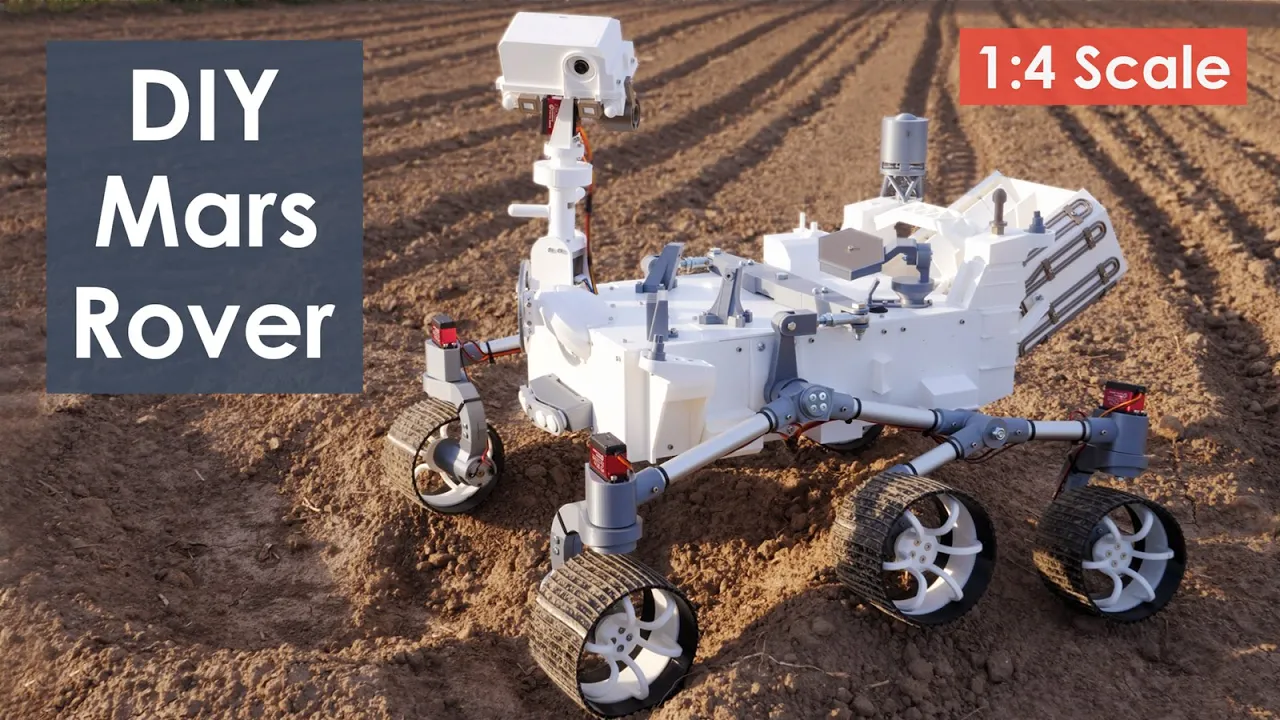
Why this video is valuable: This short, functional demonstration shows how the differential mechanism connects the left and right rocker assemblies. It showcases how a mechanical yoke or bar forces the opposite side to react inversely, stabilizing the main payload bay.
Knowledge Checkpoint
- Define why a rocker-bogie suspension system does not utilize standard springs or shocks, and state the mechanical advantage of this choice.
- Calculate how the motion of the left rocker is transferred to the right rocker via the differential bar (averaging mechanism) to stabilize the chassis pitch.
- Explain the maximum vertical obstacle clearance height of a rocker-bogie chassis in relation to its wheel diameter.
- Detail the physical load distribution change across all six wheels when the front wheel begins climbing an incline.
Module 2: CAD Design, 3D Printing, and Assembly
Translate physics into physical form. Design a custom, scale rocker-bogie suspension frame in Fusion 360, manage mechanical joint tolerances, apply structural reinforcements, and prepare parts for 3D printing.
Recommended Videos

Why this video is valuable: A complete step-by-step CAD build tutorial. It guides you through the process of sketching, projecting, and extruding the rocker, bogie, and wheel mounts inside Autodesk Fusion 360. This is the exact design pipeline needed to build the 3D-printable model files.
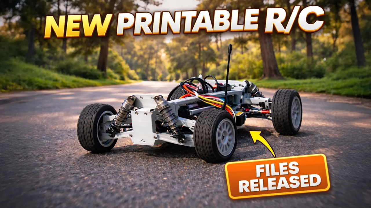
Why this video is valuable: This video focuses on practical engineering considerations for 3D-printed chassis. It covers bearing fits, joint lubrication, handling structural loads, and choosing print orientations to prevent layer delamination under bending forces.
Why this video is valuable: This tutorial illustrates structural reinforcment of 3D-printed assemblies. When building a rocker-bogie, plastic joints can easily flex or snap under torsional load. This video demonstrates how to run metal rods, bolts, or aluminum extrusions through printed elements to provide high rigidity.
Knowledge Checkpoint
- Create a kinematic sketch in Fusion 360 showing the relative pivot locations of the rocker and bogie joints, verifying joint clearance through its entire motion range.
- Determine the correct horizontal clearance (tolerances) for 3D-printed joint models to house deep-groove ball bearings without press-fit slipping.
- Explain how print orientation affects the shear strength of the primary pivot pins (layer alignment vs. torsional stress direction).
- Implement a mechanical design for the central differential pivot joint that connects the averaging bar to both the left and right rockers.
Module 3: Actuators, Power, and Microcontroller Integration
Implement control systems, power distribution, and actuation. This module deals with high-torque motor drivers, I2C PWM controllers, and the math/code needed to coordinate 6-wheel steering.
Core Concept: 6-Wheel Steering Kinematics
Standard 2WD or 4WD skid-steer setups drag wheels sideways during turns. A rocker-bogie system utilizes 4 independent corner steering servos and 6 drive motors to pivot cleanly. To avoid wheel slippage (scrubbing), you must program Ackerman Steering Kinematics extended for 6 wheels.
For any given turn angle, the rotation axes of all six wheels must intersect at a single point: the Instantaneous Center of Rotation (ICR).
   ICR (Instantaneous Center of Rotation)
    x ----------------------------------------
                            |                |
                            |                |
                      [Wheel Left Front]   [Wheel Right Front]
                         (Angle: θ_LF)        (Angle: θ_RF)
                            |                |
                            |                |
                      [Wheel Left Mid]     [Wheel Right Mid]
                         (Angle: 0)           (Angle: 0)
                            |                |
                            |                |
                      [Wheel Left Rear]    [Wheel Right Rear]
                         (Angle: θ_LR)        (Angle: θ_RR)
If the center-line wheel-to-wheel distance along the length is (front-to-mid, and mid-to-rear) and the lateral width distance is :
- Calculate the turning radius of the non-steering middle wheels from the center axis.
- Derive Steering Angles ():
- Derive Drive Wheel Velocities (): Because the wheels sit at different radial distances from the ICR, outer wheels must spin faster than inner wheels: where is the longitudinal distance from the mid-wheel line, and is the target yaw rate.
Recommended Videos
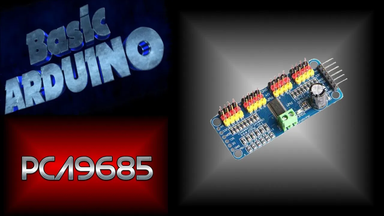
Why this video is valuable: Coordinating 4 independent corner steering servos requires precise PWM control. Standard microcontrollers do not have enough hardware timers or pins. This video demonstrates how to offload servo signals to a PCA9685 16-channel 12-bit PWM generator using a 2-pin I2C bus.
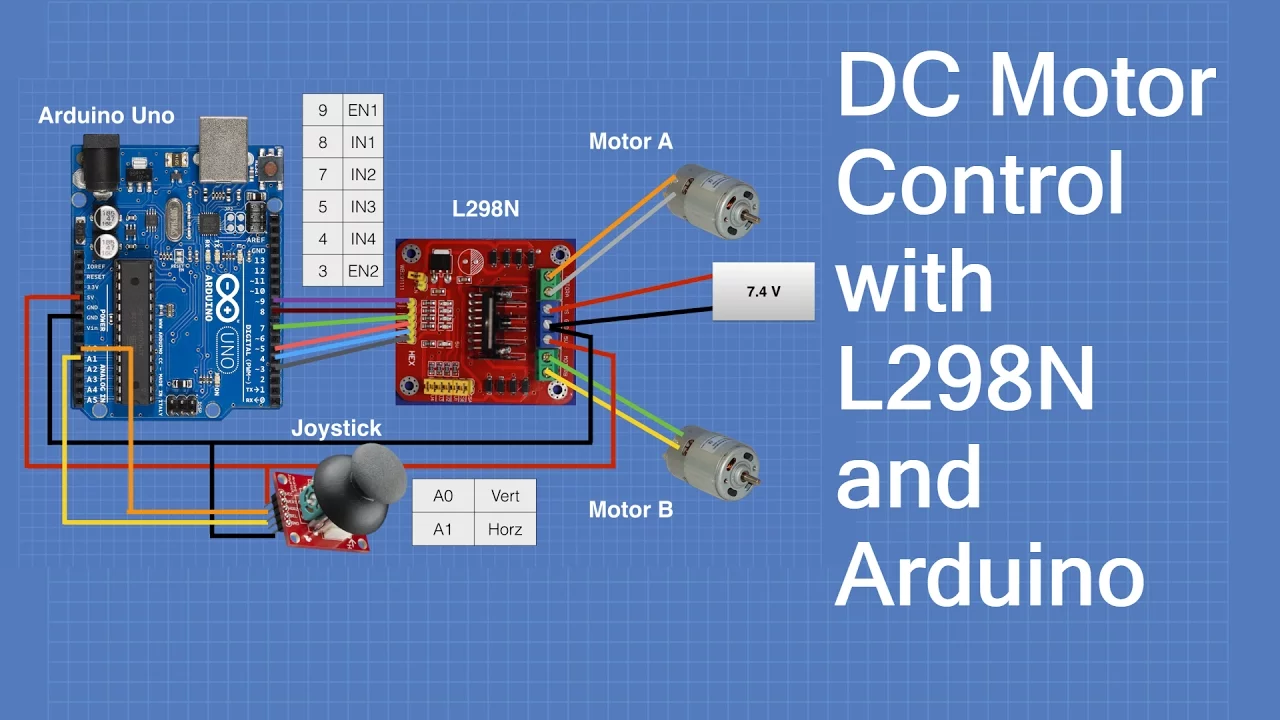
Why this video is valuable: The rover needs six high-torque DC motors driven concurrently. This guide covers using H-bridges (such as the L298N or modern equivalents) to control DC motor speed and direction using PWM and digital outputs from a microcontroller.
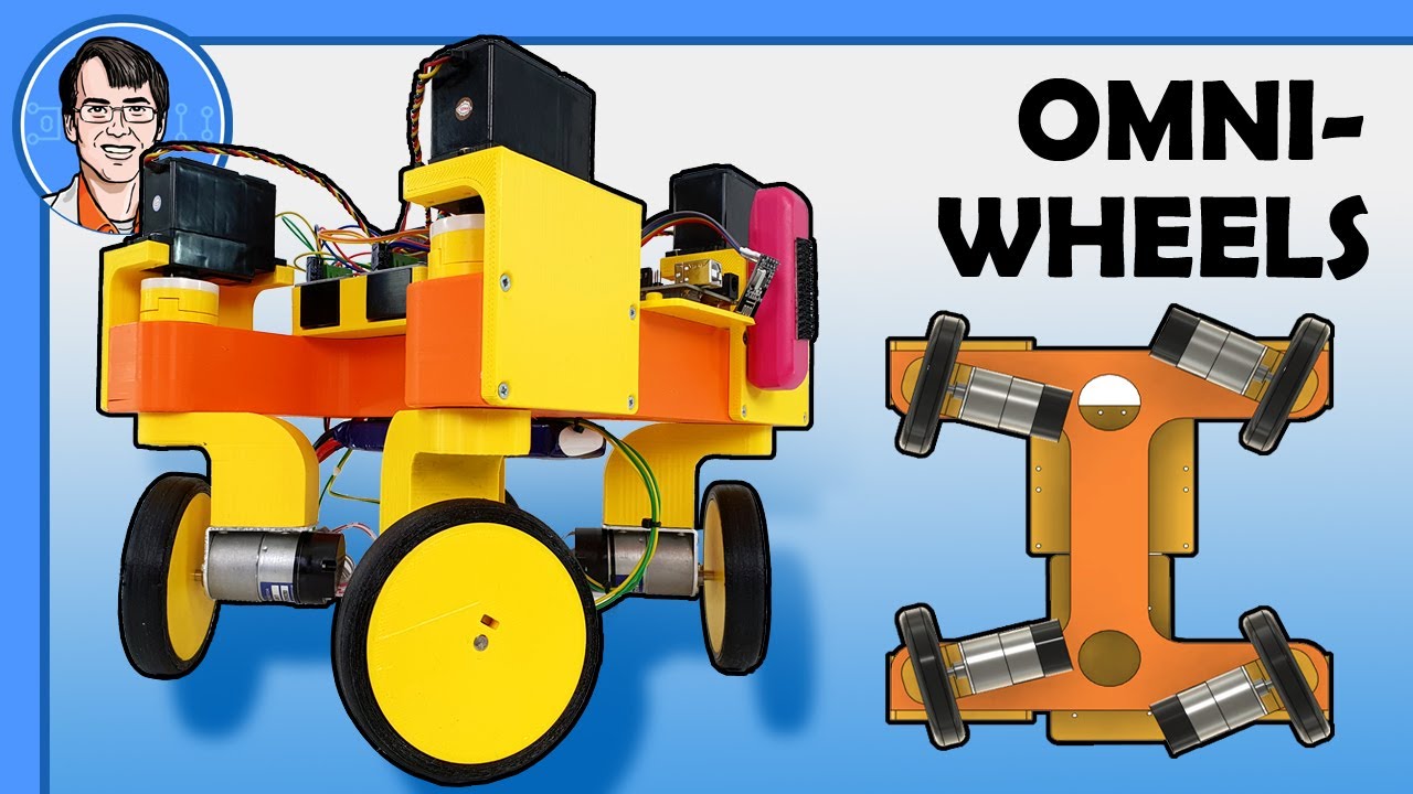
Why this video is valuable: An advanced physical look at multi-wheel steering. It details the mechanical complexity of organizing steering linkages and driving individual wheels. This visual is key to understanding why joint coordination is critical for directional alignment.
Knowledge Checkpoint
- Connect and configure the PCA9685 module over an I2C bus, setting the master frequency to 50Hz for standard analog/digital steering servos.
- Write a C++/Python function that inputs a target robot turning radius and outputs individual target angles for each of the four corner steering servos using Ackerman kinematics.
- Calculate the specific velocity scaling factors for the middle and outer wheels during a tight turn of radius .
- Create a circuit wiring diagram that correctly isolates high-current motor power from logic power, preventing microcontroller brownouts during stall currents.
Module 4: Stereo Vision and Depth Map Generation
To navigate autonomously, the rover requires local 3D perception. This module covers setting up a synchronized stereo camera rig, calibrating camera parameters, and writing software in Python to calculate disparity maps.
Mathematical Underpinnings: Disparity to Depth
Stereo cameras mimic human binocular vision. By aligning two parallel cameras separated by a baseline distance (), we can calculate the depth () of any point based on its pixel shift (disparity, ) between the two images.
              Left Camera Center        Right Camera Center
                     O_L                       O_R
                      x ----------------------- x
                      |            B            |
                      |                         |
                      |----\               /----|
                      |     \             /     |
                      |      \   Point   /      |
                      |       \    P    /       |
                      |        \ (X,Y,Z)       |
                      |         \      /        |
Left Image Plane: |--[u_l]-------/ | Right Image Plane: |------------[u_r]-------|
The projection formulas are:
The horizontal shift between corresponding projection points is called disparity ():
Thus, depth can be solved as:
Where:
- is the camera focal length (calibrated in pixels).
- is the baseline physical separation distance between camera sensors.
- is the disparity (pixel difference).
Recommended Videos
Why this video is valuable: Before estimating depth, lens distortion must be mathematically modeled and eliminated. This tutorial shows how to use a physical chessboard target to calibrate a camera, calculating the camera matrix (intrinsic parameters) and radial/tangential distortion coefficients.
Why this video is valuable:
An essential step-by-step programming guide for disparity estimation. It demonstrates how to initialize a stereo pair, perform image rectification (making the scanlines align horizontally), and configure the StereoSGBM algorithm (Semi-Global Block Matching) in OpenCV to produce real-time depth maps.
Why this video is valuable: An excellent overview of a complete, real-time object tracking and distance estimation project using stereo calibration maps. It shows the speed and accuracy of a calibrated, low-cost dual-camera assembly.

Why this video is valuable: This short comparison evaluates passive stereo depth sensors against active Time-of-Flight (ToF) cameras. It highlights why stereo cameras excel in bright outdoor settings like planetary terrains, where direct sunlight can overpower active infrared sensors.
Knowledge Checkpoint
- Perform a checkerboard camera calibration to acquire focal length () and principal point () values.
- Write an OpenCV Python script that rectifies raw left and right camera frames using calibration files so that epipolar lines are perfectly horizontal.
- Explain the inverse relationship between disparity () and depth (). What happens to the depth estimation accuracy as the object moves far away?
- Configure the parameter inputs for
StereoSGBM(such asminDisparity,numDisparities,blockSize, and smoothness penaltiesP1andP2) to minimize noise in the depth map.
Module 5: Point Cloud Processing (PCL)
Convert flat 2D depth frames into rich, spatial 3D point cloud coordinates. Isolate the traversable ground plane from vertical obstacles using geometric segmentation algorithms.
Step-by-Step Pipeline: Depth Map to Point Cloud
To convert an OpenCV depth image back to a physical 3D point cloud (), apply the inverse camera pinhole model to every pixel coordinate () holding a valid depth value :
-
Calculate Coordinate Transforms:
-
Compile Vector Matrix: Group these calculated coordinates together into a standard unstructured Point Cloud Array.
-
Execute Ground Plane Extraction (RANSAC): The RANSAC (Random Sample Consensus) algorithm iteratively models a ground plane equation:
- Step 1: Randomly select three sample points from the point cloud.
- Step 2: Compute the plane parameters .
- Step 3: Count the number of total points (inliers) that lie within a threshold distance () of this plane.
- Step 4: Repeat for iterations; the plane equation that achieves the maximum number of inliers is classified as the Ground Plane.
- Step 5: Subtract the ground points. The remaining points with coordinates above the plane are segmented as Obstacles.
Obstacle Points (High Height) * * *
------------------------------------------------- [Threshold height ε] Ground Plane Inliers (RANSAC) . . . . . .
Recommended Videos

Why this video is valuable: This tutorial bridges the gap between 2D depth maps and 3D clouds. It uses Open3D in Python to feed a depth map and its camera intrinsics into a conversion function, producing a point cloud file that can be rotated, filtered, and saved.

Why this video is valuable: This is an exceptional, fast-paced mathematical explanation of how the RANSAC algorithm operates. It explains the iterative loop of sampling, model fitting, and consensus-building that allows robots to identify geometric features amidst noisy data.

Why this video is valuable: This excerpt from an introductory point cloud course covers segmenting and isolating elements from raw collections of 3D data. It covers distance-filtering techniques and localized geometric extraction.
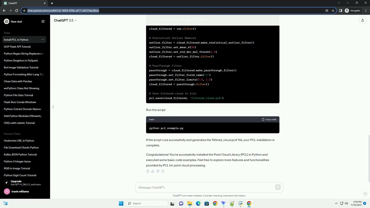
Why this video is valuable: This practical installation guide shows how to compile and load the high-performance Point Cloud Library (PCL) wrappers for Python development, establishing the local coding environment.
Knowledge Checkpoint
- Write a custom Python function to generate point cloud coordinates () from an OpenCV depth frame, using a vector-mapped NumPy algorithm rather than slow pixel-by-pixel loops.
- Install the Open3D/PCL library and verify point cloud loading and display capabilities using standard PLY/PCD formats.
- Write a script to isolate the ground plane from a 3D scene using a custom RANSAC plane-segmentation loop, outputting the remaining obstacle-only points.
- Implement voxel grid downsampling on a raw point cloud to reduce computational load without losing critical obstacle boundaries.
Module 6: Autonomous Path Planning and Obstacle Avoidance in ROS
Integrate physical actuation, kinematic control, and 3D perception into the Robot Operating System (ROS). Feed point clouds into local costmaps to allow autonomous, collision-free obstacle negotiation.
Core Concept: Custom Point Cloud Costmap Integration
The ROS Navigation Stack (Move Base / Nav2) handles obstacle avoidance using 2D or 3D costmaps. To feed custom point clouds (sensor_msgs/PointCloud2) directly into costmaps for local path planning:
              [Custom Stereo Vision Node]
                           |
               (sensor_msgs/PointCloud2)
                           |
                           v
                 [ROS Navigation Node]
               (Costmap_2D Obstacle Layer)
                           |
         /-----------------+-----------------\
        |                                     |
        v                                     v
 [Local Costmap]                      [Global Costmap]
(Dynamic local obstacles) (Static base map files) | | -----------------+-----------------/ | v [Local Path Planner] (e.g., DWA / TEB) | (geometry_msgs/Twist) | v [6-Wheel Steering Controller]
- Configure the Obstacle Layer inside your local costmap configuration YAML parameters file:
local_costmap: obstacle_layer: observation_sources: stereo_cloud stereo_cloud: sensor_frame: camera_link data_type: PointCloud2 topic: /stereo_camera/point_cloud marking: true clearing: true min_obstacle_height: 0.1 max_obstacle_height: 1.0 obstacle_range: 2.5 raytrace_range: 3.0 - Execute Obstacle Processing: Setting
marking: trueinserts points within the height threshold into the grid as lethal navigation barriers. Settingclearing: trueclears barriers when the sensor's line-of-sight passes through that space without hitting anything. - Generate Velocity Commands: The local path planner (like DWA or TEB) tracks these costmap updates and outputs target linear/angular velocities (
geometry_msgs/Twist). - Distribute Kinematics: The custom motor controller driver intercepts this command and runs the 6-wheel Ackerman equations to move the rover safely around obstacles.
Recommended Videos
Why this video is valuable: An excellent, exhaustive reference guide on configuring costmaps, setting robot dimensions, and tuning navigation behaviors inside the ROS Navigation architecture. It details how the robot maintains situational awareness by combining sensor updates with environmental maps.

Why this video is valuable: This practical, physical demo showcases a mobile robot navigating around obstacles in real-time. It provides a visual walk-through of the complete ROS network, showing how the local path planner alters velocities dynamically as obstacles appear.

Why this video is valuable: This real-world implementation demonstrates feeding low-cost synchronized stereo camera inputs into RTAB-Map ROS to construct highly accurate, spatial point clouds and local grid maps.
Knowledge Checkpoint
- Launch the ROS Navigation core and verify that custom coordinate frames (such as
odom,base_link, andcamera_link) are correctly linked in your TF transform tree. - Configure the local costmap configuration file to subscribe to
/stereo_camera/point_cloudas an active obstacle observation source. - Write a custom ROS subscriber node that takes in standard
/cmd_vel(Twist) commands and publishes matching wheel speed and steering angle configurations to your actuators. - Tune costmap inflation radius values to ensure the six-wheeled rover maintains a safe physical clearance distance from obstacles.
Course Map
Key People Index
- Donald Bickler
- Context: The principal mechanical engineer at NASA JPL who invented and patented the rocker-bogie suspension system, facilitating NASA's planetary exploration beginning with the Sojourner rover.
- Cyrill Stachniss
- Context: Renowned robotics professor and researcher specializing in mobile robotics, photogrammetry, mapping, and SLAM. His educational lectures serve as the industry baseline for mathematical algorithms like RANSAC.
- Nicolai (NicolaiAI)
- Context: Practical robotics engineer and computer vision educator whose detailed guides walk developers through camera calibration, rectification, and block matching in OpenCV.
- James Bruton
- Context: Creative robotics developer and former toy designer who builds and documents complex, open-source mechanical systems, motor configurations, and ROS integrations.
Final Self-Assessment
Complete this comprehensive self-assessment to verify your mastery of the rocker-bogie autonomous navigation pipeline:
- Structural Assembly: Construct a physical 6-wheeled rocker-bogie chassis where all joint pivots swing freely and the central differential bar balances rocker pitch changes.
- Actuation Control: Connect all six drive motors and four corner steering servos to your controller via the PCA9685, verifying that each joint can be addressed individually.
- Kinematic Logic: Implement the mathematical 6-wheel Ackerman equations in firmware so that steering angles adjust relative to a target Instantaneous Center of Rotation (ICR) without any wheel drag.
- Camera Calibration: Calibrate a dual-camera setup using chessboard-pattern targets, achieving a projection reprojection error under 0.5 pixels.
- Depth Reconstruction: Write a Python script to compute stereo disparity maps in real-time, outputting clean depth measurements of nearby objects.
- Point Cloud Conversion: Convert depth maps to structured 3D coordinates () using coordinate transform projection matrices.
- RANSAC Segmentation: Apply the RANSAC algorithm to segment the ground plane, successfully separating flat, traversable ground from high-elevation obstacles.
- Costmap Population: Feed your obstacle-only point cloud directly into the ROS local costmap as a
/sensor_msgs/PointCloud2topic, marking obstacle coordinates as navigation barriers. - Closed-Loop Navigation: Send a navigation target coordinate to the ROS navigation stack and verify that the rover calculates a safe path, commands steering servos, and navigates around obstacles without colliding.