This video demonstrates how to perform 3D mapping using RTAB-MAP-ROS with a synchronized USB stereo color global shutter camera (SVPRO 3200x1200@5fps, M12, 85deg FOV), showing the integration of consumer-grade vision hardware with robotics mapping software for real-time environmental reconstruction.
Stereo Camera Mapping with RTAB-Map ROS Tutorial
Added:Deep Dive
Basic proficiency in ROS (Robot Operating System) concepts, including nodes, topics, messages, tf transformations, and launch files.
Introduction to ROS Part 1: What is the Robot Operating System? | DigiKey
40.5K
ROS (Robot Operating System) is an open-source middleware framework that sits between the underlying operating system and robot application code, breaking robot code into manageable nodes. The fundamental building block is a node—a process performing tasks like sensor reading or motor control. Nodes communicate via topics (publish-subscribe model) and services (synchronous request-response). All messages use strongly typed interfaces defining data formats. ROS encourages splitting nodes into separate files for readability and reusability. Micro-ROS exists as a lightweight version for microcontrollers, integrating with real-time OSes like FreeRTOS and Zephyr.
Click to watch →
![[GHW Open Source] Getting started with ROS 2 for Open Source projects](https://i.ytimg.com/vi/8pZYK6qACH0/maxresdefault.jpg)
[GHW Open Source] Getting started with ROS 2 for Open Source projects
343
ROS 2 has several core concepts: Workspaces are directories storing all files and packages; Packages are organization units containing nodes, messages, and launch files; Nodes are small focused programs performing specific tasks like sensor reading or motor control; Topics are channels for continuous data streaming where nodes publish and subscribe to messages; Messages are data structures carrying information over topics; Services implement synchronous request-response communication between nodes. These concepts enable modular robot development where different components communicate efficiently.
Click to watch →

Getting Started with ROS Part 1: Nodes, Parameters and Topics
23.2K
ROS (Robot Operating System) programs robots using five core constructs: Nodes (single-purpose processing modules that serve as graph vertices), Parameters (name-value pair configuration items set at startup), and Topics (edges that enable flexible publisher-subscriber communication between nodes); nodes handle computation while topics broker data flow using predefined message types, allowing robots to be represented as dynamic directed graphs that can span multiple computers.
Click to watch →

ROS Basics in Ubuntu 18.04: Node, Messages, Topic, Publisher and Subscriber
7.3K
In ROS (Robot Operating System), a node is an executable file (Python or C++ script) that performs specific functions; messages are data structures (integers, floats, strings, characters) used for communication between nodes; topics are communication channels that enable multiple nodes to share data efficiently; publishers send data to topics, while subscribers receive data from topics, enabling one-to-many communication patterns that optimize data distribution across multiple nodes.
Click to watch →
![[UDEMY COURSE] ROS Tutorial 2: Understanding ROS Topics, Node and Messages](https://i.ytimg.com/vi/Yx_vGAt74sk/sddefault.jpg)
[UDEMY COURSE] ROS Tutorial 2: Understanding ROS Topics, Node and Messages
67.1K
In ROS (Robot Operating System), nodes are independent processes that communicate through topics (named channels for data exchange) and messages (structured data units). To launch a ROS node, use the 'ros run' command followed by the package name. Nodes can publish messages to topics and subscribe to topics from other nodes, enabling distributed robot control. The 'ros node list' command displays all running nodes, while 'ros topic list' shows available topics. The 'ros node info' command provides detailed information about a specific node, including its published and subscribed topics.
Click to watch →
Deep Dive
Fundamental understanding of stereo vision, including epipolar geometry, disparity maps, depth estimation, and camera calibration.
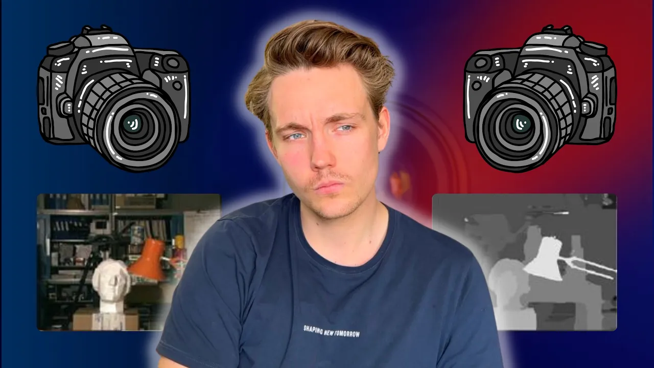
Stereo Vision and Depth Estimation Using OpenCV (C++ & Python)
86.1K
Stereo vision uses two synchronized cameras to estimate depth by calculating disparity—the horizontal difference in image positions of corresponding points between the two views—through epipolar geometry, enabling 3D reconstruction of scenes and distance estimation to objects; this is achieved by first calibrating both cameras to obtain intrinsic and extrinsic parameters, then computing disparity maps via block matching along epipolar lines, and finally converting disparity to depth using the formula depth = (focal_length × baseline) / disparity.
Click to watch →
Extra Session: Computer Vision | NPTEL noc25-cs143 Full Discussion
311
This section covers stereo geometry using two cameras to recover depth information. Key concepts include epipolar geometry, fundamental matrix (F) and essential matrix (E), and depth computation formula (depth = KTX/(X-X')). The section also covers parametric representation of fundamental matrix and retrieving camera matrices from fundamental matrix. These concepts are fundamental for 3D vision and depth estimation applications.
Click to watch →
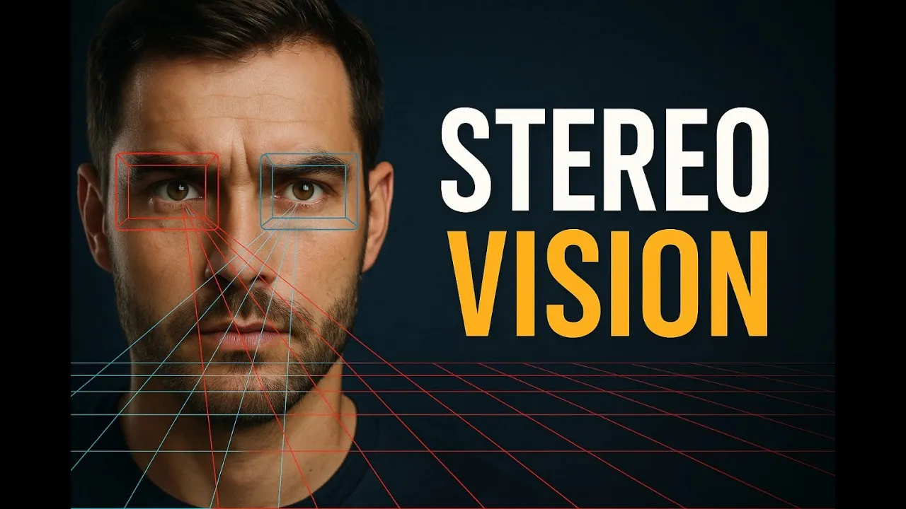
Stereo Vision Explained: How Depth Perception Works in Computer Vision
692
Stereo vision enables machines to perceive depth by comparing two images captured from slightly different viewpoints using two cameras, where closer objects appear more shifted (higher disparity) and distant objects appear less shifted, allowing computation of depth through disparity maps via triangulation using the formula depth = (focal length × baseline) / disparity, with applications spanning autonomous driving, robotics, and augmented reality.
Click to watch →
Stereo 3D Vision (How to avoid being dinner for Wolves) - Computerphile
149.5K
Stereo 3D vision uses two cameras positioned at known locations to reconstruct 3D scenes by finding corresponding points between left and right images; the key mathematical concept is epipolar geometry, which restricts the search for matching points to specific lines (epipolar lines) rather than the entire image, making the correspondence problem computationally tractable.
Click to watch →

CVFX Lecture 14: Epipolar geometry
50.7K
Epipolar geometry describes the geometric relationship between two images of the same scene captured from different viewpoints. Unlike optical flow which allows correspondences anywhere in the image, epipolar geometry constrains correspondences to specific lines called epipolar lines. The baseline connects the two camera centers, and a family of planes pivoting around this baseline generates conjugate epipolar line pairs. Every point on one line corresponds to a point on its conjugate line in the other image. This transforms the 2D correspondence problem into a series of 1D searches, making correspondence finding computationally more efficient and enabling more accurate matching algorithms.
Click to watch →
Deep Dive
Core concepts of SLAM (Simultaneous Localization and Mapping), particularly visual odometry and the role of loop closure detection.

Self-Driving Cars - Lecture 7.2 (Odometry, SLAM and Localization: SLAM)
4.7K
Simultaneous Localization and Mapping (SLAM) optimizes over the entire history of recorded frames rather than just adjacent frames, jointly optimizing camera poses and 3D feature locations. Unlike visual odometry where the map is a by-product, SLAM addresses the chicken and egg problem where accurate localization requires accurate mapping and vice versa. Loop closure detection corrects drift by matching features across distant frames when revisiting locations. Feature-based SLAM uses bundle adjustment to minimize reprojection errors—the distance between observed image features and projected 3D points—optimizing both extrinsic and intrinsic camera parameters along with 3D landmark locations.
Click to watch →
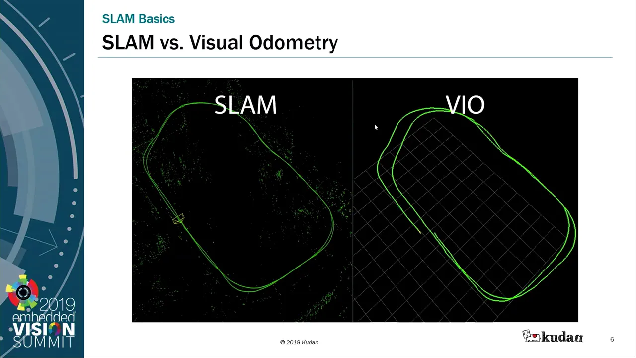
Commercial Grade SLAM Frameworks for Indoor and Outdoor Applications a Presentation from Kudan
5.2K
Loop closure is the secret weapon of SLAM systems. It enables the system to recognize when it has returned to a previously mapped area. When this recognition occurs, the system can measure the accumulated drift that has existed throughout tracking and then close the loop to correct the error. This capability results in far more accurate maps than visual odometry systems can achieve, as it provides a mechanism to correct accumulated errors over time.
Click to watch →

Robust and Efficient Visual SLAM (Andrew Calway / University of Bristol, UK)
2.1K
Loop closure is a critical mechanism in Visual SLAM that corrects accumulated drift. When the camera returns to a previously visited location and recognizes features seen earlier, it can correct not just the current pose but all previous estimates in a domino effect. Without loop closure, the system will continue drifting indefinitely. Loop closure can be implemented locally (returning to nearby positions) or globally (returning to distant starting points).
Click to watch →
Simultaneous Localization And Mapping (SLAM)
25.7K
Loop closure is a stage in SLAM that identifies when an agent has returned to a previously visited location. For example, if someone walks around a room and returns to their starting point, loop closure helps establish that this is not a new area but rather a previously mapped location. This prevents the system from creating duplicate maps of the same space.
Click to watch →

Lec-10: Graph-Based SLAM (English)
102
Loop closure is the process of recognizing when the robot has come back to a previously visited location. This allows us to create a new constraint that helps pull the current estimated pose back toward where it should be, reducing accumulated error. When the robot returns to a previously visited location, both scans observe the same part of the map, so we can connect these two poses with a loop closure constraint. A good way to visualize this is by imagining a virtual spring between the two poses that wants to pull them together because they ideally represent the same location.
Click to watch →
Deep Dive
Familiarity with sensor hardware concepts, specifically the difference between global shutter and rolling shutter cameras.

Raspberry Pi fixed the rolling shutter problem
114K
Rolling shutter cameras read sensor pixels line-by-line, causing distortion when capturing moving subjects or camera movement (the 'Jello effect'), while global shutter cameras capture all pixels simultaneously using a special buffer, eliminating distortion but typically requiring lower resolution or higher cost.
Click to watch →
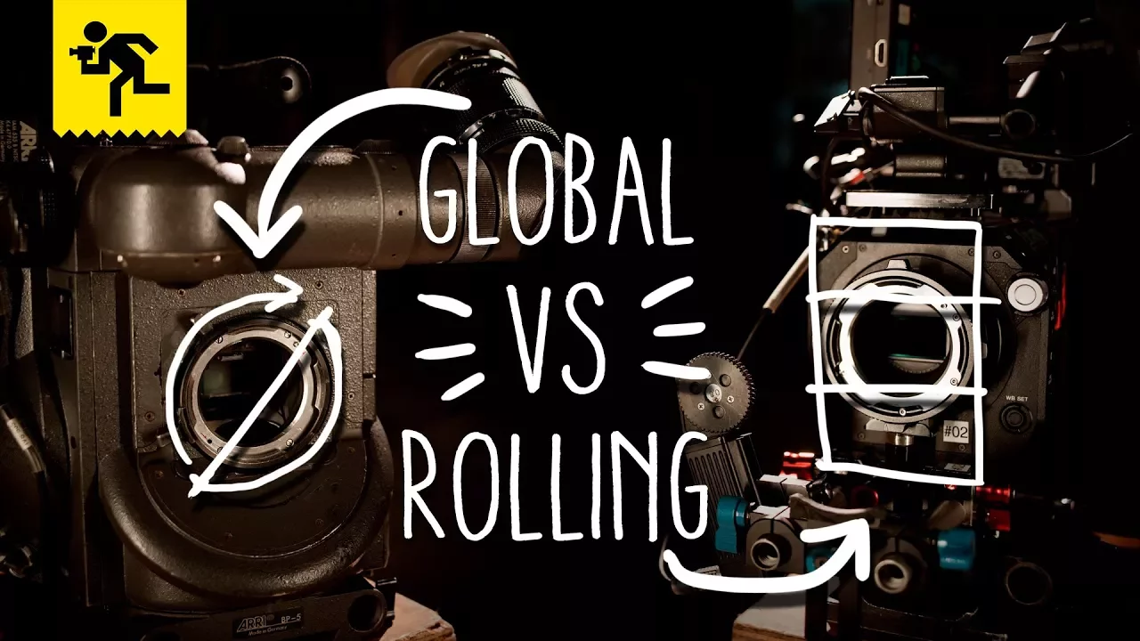
FOTOGRAFIA - QUAL A DIFERENÇA ENTRE GLOBAL SHUTTER E ROLLING SHUTTER?
25.8K
Global shutter captures an entire image simultaneously by enabling and disabling all sensor pixels at once, while rolling shutter exposes the sensor sequentially from top to bottom, which can cause motion distortion when subjects move faster than the exposure rate.
Click to watch →

Global Shutter vs. Rolling Shutter - What's the difference? (ft. SONY A9iii)
13K
Rolling shutter cameras expose the sensor progressively line-by-line from top to bottom, causing moving objects to appear distorted or warped, while global shutter cameras expose the entire sensor simultaneously, eliminating distortion and banding effects; the Sony A9 Mark II represents the first consumer-level global shutter full-frame mirrorless camera, enabling faster readout speeds that make it ideal for high-speed photography and video without the warping effects seen in rolling shutter cameras.
Click to watch →

Global Shutter, la revolución que viene (¿o no es para tanto?)
62.5K
A global shutter captures information from all photodiodes of all pixels in the sensor simultaneously, meaning all pixels are activated at the same time. In contrast, a rolling shutter (used in CMOS sensors) performs a sequential scan by lines, which creates the characteristic image distortion known as the 'gelatin effect' when capturing moving objects.
Click to watch →

If Zuckerberg Hides His Kids' Faces in Photos... Should YOU? | The PetaPixel Podcast
17.3K
Rolling shutter and global shutter represent fundamental differences in how image sensors capture light. Rolling shutter scans sensors line by line, causing distortion during fast movements, while global shutter captures all pixels simultaneously. Each approach involves trade-offs: rolling shutter offers better dynamic range and lower cost, while global shutter eliminates motion artifacts. Modern stacked sensor designs attempt to balance these competing priorities, representing ongoing technological evolution in imaging hardware.
Click to watch →
Prerequisite Knowledge
- Concept 01Basic proficiency in ROS (Robot Operating System) concepts, including nodes, topics, messages, tf transformations, and launch files.
- Concept 02Fundamental understanding of stereo vision, including epipolar geometry, disparity maps, depth estimation, and camera calibration.
- Concept 03Core concepts of SLAM (Simultaneous Localization and Mapping), particularly visual odometry and the role of loop closure detection.
- Concept 04Familiarity with sensor hardware concepts, specifically the difference between global shutter and rolling shutter cameras.
Subsequent Learning
- Step 01Integrating the generated 3D occupancy grid with the ROS Navigation Stack (Move Base or Nav2) for autonomous path planning and obstacle avoidance.
- Step 02Advanced optimization of RTAB-Map parameters, such as tuning loop closure heuristics, feature detectors, and memory-management constraints for large-scale environments.
- Step 03Implementing Visual-Inertial Odometry (VIO) by fusing stereo camera feeds with IMU (Inertial Measurement Unit) data for robust tracking in low-texture scenes.
- Step 04Deploying and optimizing 3D mapping algorithms on embedded edge computing platforms (e.g., NVIDIA Jetson) for mobile robotics applications.
Core Concept
Core Concept
0:02Playing Section
- 1
Introduces the main topic directly.
- 2
Highlights the speed of the core idea.
- 3
Sets the stage for deeper discussion.
Active Sensing and LiDAR-Based SLAM
While stereo camera mapping with RTAB-Map is a cost-effective and feature-rich visual SLAM solution, it has significant limitations compared to active sensing methods like LiDAR-based SLAM (e.g., Cartographer, LOAM). Passive stereo vision relies heavily on ambient lighting and rich visual textures to extract features. In low-light conditions, glare, or featureless environments like long corridors and uniform walls, visual SLAM often fails due to tracking loss. In contrast, LiDAR emits its own light, providing highly accurate, direct 3D range measurements regardless of lighting or texture. Furthermore, processing high-resolution stereo images for feature extraction and depth estimation is computationally intensive, whereas LiDAR-based approaches offer direct geometric data, reducing CPU load. For critical industrial applications demanding high precision, reliability, and safety, LiDAR remains the industry standard, making it a vital alternative perspective to purely visual mapping approaches.
Deep Dive
Integrating the generated 3D occupancy grid with the ROS Navigation Stack (Move Base or Nav2) for autonomous path planning and obstacle avoidance.
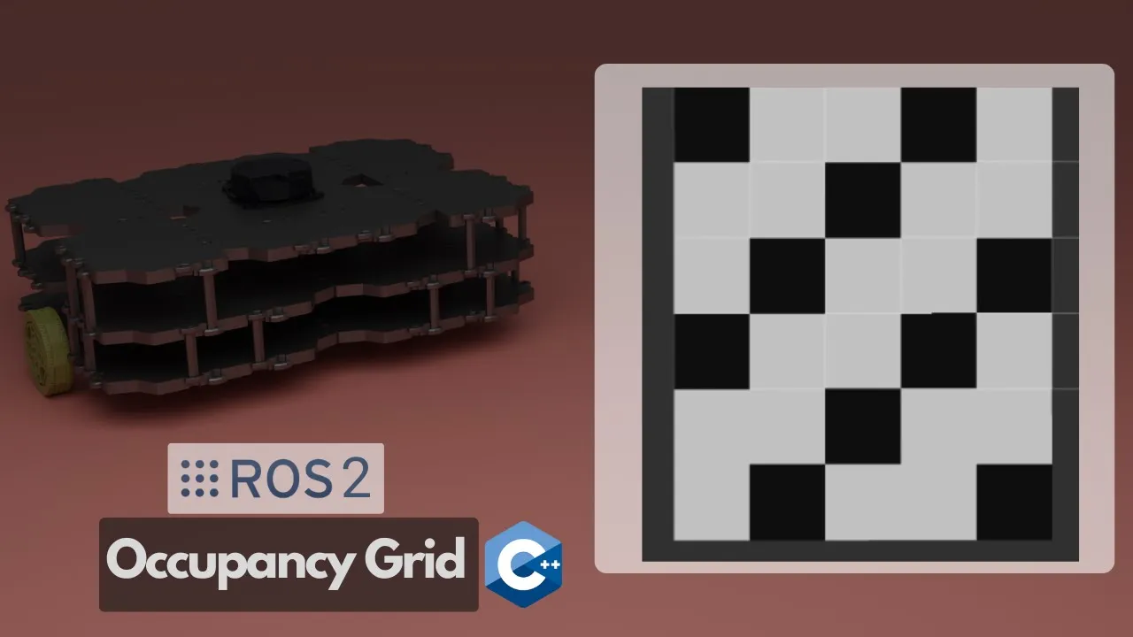
ROS2 Occupancy Grid Node for Nav2
13.4K
An occupancy grid is a fundamental data structure in robotics that represents a 2D environment as a grid of cells, where each cell contains an integer value indicating its state: 100 represents occupied/obstacle, 0 represents free space, and -1 represents unexplored areas; this node demonstrates how to publish such a grid in ROS2 using C++ by creating a custom publisher that constructs and populates the nav_msgs/OccupancyGrid message with appropriate header information, frame ID, resolution, origin, height, width, and the data array containing the grid values, enabling the creation of artificial maps for path planning algorithms.
Click to watch →
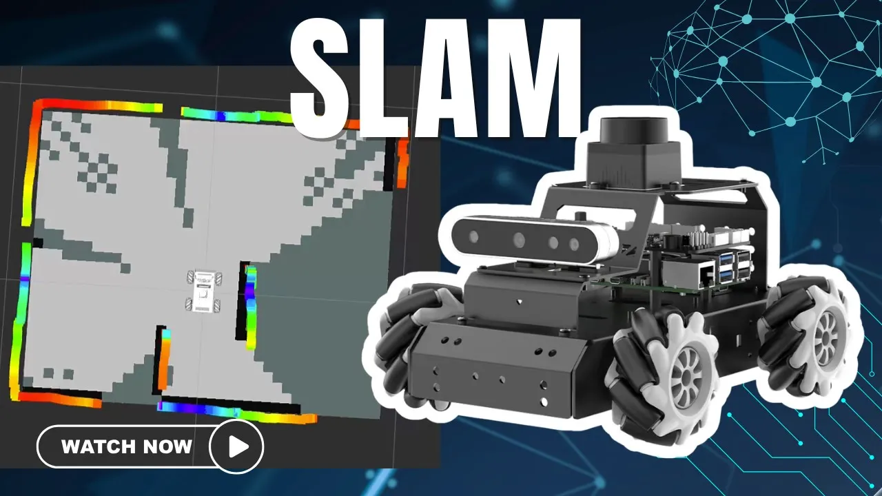
ROS2 SLAM & Navigation Demo: MentorPi M1 Raspberry Pi 5 Robot Autonomous Maze Navigation
6.2K
SLAM (Simultaneous Localization and Mapping) enables robots to build real-time 2D occupancy grid maps while simultaneously determining their own position using sensor data like LiDAR point clouds, processed through algorithms that pre-process observations, match them with existing maps, and fuse new data to update the map; this mapping capability then feeds into the ROS2 Nav2 navigation stack, which uses global path planning, local planners like DWA (Dynamic Window Approach), and AMCL (Adaptive Monte Carlo Localization) to enable autonomous single and multi-point navigation with obstacle avoidance and recovery behaviors.
Click to watch →

Autonomous Navigation Mobile Robot using ROS | Jetson Nano | RPLidar | Differential Drive Kinematics
162.2K
This video demonstrates how to implement autonomous navigation for a differential drive mobile robot using the ROS navigation stack, covering the key components including the map server for providing environment maps, AMCL node for robot localization using sensor data, move_base node for path planning and obstacle avoidance, and the differential drive controller for converting velocity commands to wheel velocities; the tutorial shows practical implementation steps including 3D printing the robot chassis, configuring the differential drive controller with parameters like wheel separation and radius, performing SLAM mapping using rplidar, and achieving autonomous navigation where the robot successfully navigates to goal locations while avoiding obstacles.
Click to watch →
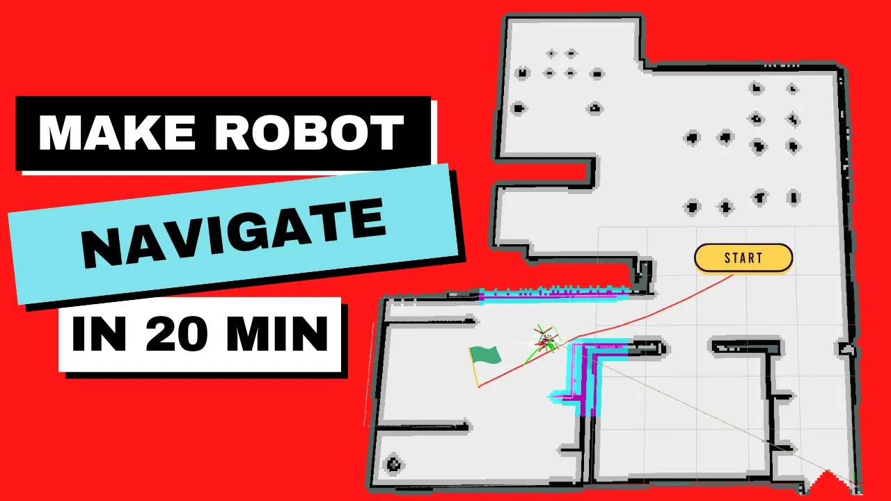
Navigation simulating | Movebase : Navigation Framework for ROS | Costmap | Planner | Part 5
33.4K
Move_base is a versatile ROS navigation framework that enables autonomous robot navigation by integrating global and local planners with costmaps; it works by taking a map from a map server, using a global planner (like navfn) to compute a global path to the goal, then using a local planner (like trajectory_planner) with sensor data and local costmaps to generate velocity commands for obstacle avoidance, allowing robots to navigate from point A to point B autonomously.
Click to watch →
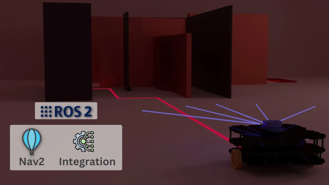
Nav 2 in ROS 2 for autonomous Navigation using SLAM for Indoor Mobile Robots
32.1K
The ROS 2 Nav2 stack enables indoor mobile robots to achieve autonomous navigation by integrating four key components: AMCL (Monte Carlo localization) for robot positioning, BT Navigator for behavior tree-based path planning, cost maps (global and local) for obstacle avoidance, and planners (like DWB) for motion generation. The system works by first creating a 2D occupancy grid map using SLAM techniques with LIDAR and odometry data, then using this map along with real-time sensor data to plan paths and navigate to goals autonomously. Multiple goals can be sent sequentially through the navigation stack, enabling waypoint navigation where the robot automatically travels through a series of designated points.
Click to watch →
Deep Dive
Advanced optimization of RTAB-Map parameters, such as tuning loop closure heuristics, feature detectors, and memory-management constraints for large-scale environments.
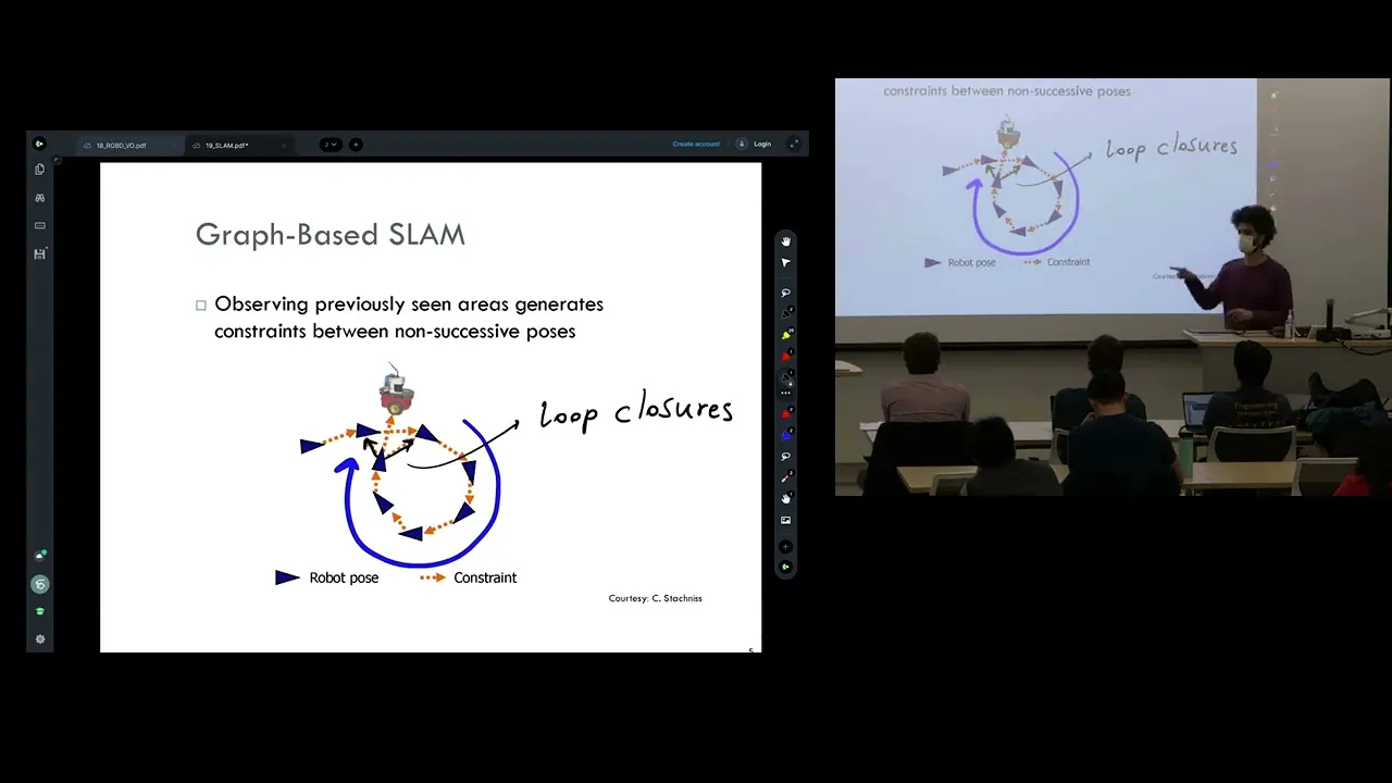
Lecture 19-SLAM I
2.1K
Searching for loop closures among thousands of nodes is combinatorial and exponentially grows. Practical solutions include: (1) Using a map to limit search to the robot's neighborhood; (2) Using semantic knowledge (like recognizing rooms or areas) to guide data association; (3) Visual place recognition methods like bag of words, which convert images to visual word histograms and compare against a library to find matches.
Click to watch →
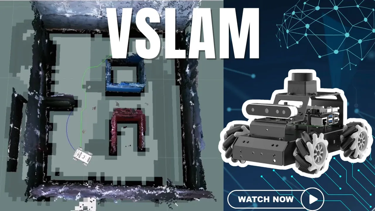
Visual SLAM VSLAM ROS2 Demo: 3D Mapping & Autonomous Navigation using MentorPi M1 Raspberry Pi 5
412
RTAB-VSLAM (Realtime Appearance-Based Visual Simultaneous Localization and Mapping) is an open-source library that creates 3D maps while simultaneously tracking robot position in real time. The system employs intelligent memory management with two distinct memory types: short-term memory handles continuous data matching for real-time map building, while long-term memory detects loop closures when the robot revisits previously seen areas, ensuring fixed-time processing for large-scale environments. The feature-based mapping algorithm extracts distinctive visual features from camera images, matching them across timestamps to detect environmental changes. Short-term memory updates positioning points dynamically, while long-term memory integration improves accuracy when matching future data. Best practices for optimal mapping include reducing robot speed to minimize odometry error, starting mapping near straight walls or enclosed areas, performing complete 360° scans, and completing full mapping loops before focusing on details. The system automatically saves maps upon session termination.
Click to watch →
![[ROS tutorial] RTAB-Map in ROS 101](https://i.ytimg.com/vi_webp/gJz-MWn7jhE/maxresdefault.webp)
[ROS tutorial] RTAB-Map in ROS 101
41K
Autonomous navigation requires creating a map first. The mapping process involves launching RTAB-Map alongside the move_base node from the navigation stack, with the grid map topic remapped to the move_base node's map topic parameter. The robot explores the environment using keyboard teleop, and RViz visualizes the map creation process. After mapping, all data is stored in a database containing images with yellow disks indicating key features (corners, intersections, distinctive objects). The database viewer displays images chronologically. Pink disks indicate loop closures - when two images share matching key features, the system detects the robot has returned to a previously visited location, enabling position correction and accurate long-term mapping.
Click to watch →
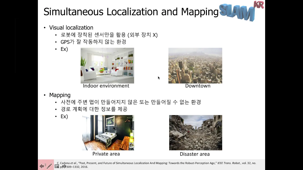
20190106 Introduction to SLAM
13.6K
Back-end optimization addresses accumulated drift errors using loop closure information. The system identifies when the robot returns to previously visited locations and uses this constraint to globally optimize the trajectory. Two main approaches exist: filter-based methods (Kalman Filters, Particle Filters) and optimization-based methods (Bundle Adjustment, Pose Graph Optimization). Optimization-based methods have become dominant due to improved computing power and the ability to exploit sparsity in the problem structure. Loop closure detection compares current sensor data with historical data to identify matching locations, enabling global trajectory correction and consistent map generation.
Click to watch →

RI Seminar: Michael Kaess: Factor Graphs for Robot Perception
12.4K
When the robot returns to an area it has previously scanned, overlapping submaps can be registered together to create loop closure constraints. This registration process determines the offset between poses from different submaps, providing additional constraints that eliminate drift. The resulting graph is called a pose graph because it only involves poses and constraints between them, without explicitly modeling landmarks, reducing optimization complexity.
Click to watch →
Deep Dive
Implementing Visual-Inertial Odometry (VIO) by fusing stereo camera feeds with IMU (Inertial Measurement Unit) data for robust tracking in low-texture scenes.

Metric-Semantic SLAM with Kimera: A Hands On Tutorial
17.9K
Kimera-VIO implements Visual-Inertial Odometry (VIO) by fusing stereo camera data with IMU measurements to estimate 3D robot poses and reconstruct 3D landmarks. The system operates as two components: a standalone C++ library containing core mathematical algorithms, and a thin ROS wrapper for interfacing. The pipeline processes stereo images, extracts visual features, tracks them across frames, and estimates the camera trajectory in real-time. Feature states are visualized with color coding: red for undetected features, blue for tracked features below threshold, and green for reliable tracked features. Users can switch between point cloud and mesh visualization modes during runtime. The output provides sparse point cloud representations suitable for obstacle avoidance applications.
Click to watch →

L16 Introduction to Visual SLAM
12.3K
Visual-Inertial Odometry (VIO) combines visual SLAM with IMU (Inertial Measurement Unit) measurements through tight sensor fusion in a unified optimization framework. The system jointly optimizes camera poses, 3D landmarks, IMU biases, and velocities within a factor graph. This approach leverages the complementary strengths: cameras provide absolute position and landmark observations, while IMUs provide reliable short-term orientation and acceleration measurements. Estimating IMU biases continuously is critical because uncorrected biases cause rapid divergence. The scale ambiguity of monocular vision is resolved using accelerometer measurements over time.
Click to watch →
Robust, Visual-Inertial State Estimation: from Frame-based to Event-based Cameras
32.3K
Visual-inertial fusion combines camera and IMU measurements to estimate robot state (position, velocity, biases). The mathematical formulation involves solving for unknowns including absolute scale and IMU biases using inertial and visual measurements. Martinelli's work enables closed-form initialization from three consecutive views with sufficient acceleration. Two implementation strategies exist: filter-based methods (MSCKF) tracking ~20 features for efficiency versus optimization-based approaches maintaining sliding windows or full trajectories for higher accuracy. The choice depends on real-time performance versus accuracy trade-offs, with optimization approaches using iSAM achieving real-time operation at 50Hz through incremental updates.
Click to watch →

Robust Stereo Visual Inertial Odometry for Fast Autonomous Flight
16.6K
This video demonstrates a stereo Multi-State Constraint Kalman Filter (MSCKF) based Visual-Inertial Odometry (VIO) system that achieves robust state estimation for autonomous flight, showing successful navigation through unstructured environments with drift of only 0.5% over 700-meter trajectories while maintaining computational efficiency comparable to state-of-the-art monocular solutions.
Click to watch →

Towards End to end Learning of Visual Inertial Odometry with an EKF
1.8K
This section introduces the core motivation and methodology for combining deep learning with classical state estimation in VIO. Monocular VIO uses one camera and IMU to improve performance and robustness over classical methods that rely on manually crafted pipelines prone to errors in rapid motion, exposure changes, and low texture environments. The proposed approach uses a robocentric EKF where the IMU kinematic model provides prediction, while learned relative poses and covariances enable measurement updates. This hybrid architecture leverages deep learning's strength in handling high-dimensional image data while maintaining the physical plausibility of classical EKF frameworks.
Click to watch →
Deep Dive
Deploying and optimizing 3D mapping algorithms on embedded edge computing platforms (e.g., NVIDIA Jetson) for mobile robotics applications.

GTC 2019 Keynote with NVIDIA CEO Jensen Huang
219.8K
The Jetson Nano is NVIDIA's smallest computer at $99, running the entire CUDA-X stack including computer vision and speech recognition. It enables 200,000 developers across 2,000 companies to build robots for warehouse logistics, agriculture, retail, and industrial applications. The Isaac robotics platform provides three reference robots (Kaya, Carter, Link), a robotic simulator for virtual training, and tools for reinforcement learning. NVIDIA DRIVE is an autonomous vehicle platform consisting of: DGX Saturn 5 supercomputer for AI training, ensemble AI algorithms for perception/localization/path planning, DRIVE AV Constellation simulation platform for testing corner cases, and DRIVE IX for human-machine interface. Release 9 provides Level 2 capabilities including off-ramp/on-ramp, auto lane change, real-time mapping, and driver monitoring.
Click to watch →
Bringing Generative AI to Life with NVIDIA Jetson
25.3K
This video demonstrates how NVIDIA Jetson enables deployment of large language models (LLMs) and vision transformers (VITs) at the edge through optimized software stacks (Jetpack 6), quantization techniques (4-bit quantization reduces 70B LLM memory from 140GB to ~35GB), and integrated tools like TensorRT, Riva for speech, and Isaac ROS for robotics, achieving real-time performance (95 FPS for VITs, interactive rates for LLMs) while maintaining low latency, privacy, and offline operation for applications like robotics and autonomous systems.
Click to watch →

Building an AI Robot that can be trained! || Using an NVIDIA single board computer
352.5K
This video demonstrates how to build an autonomous AI robot using an NVIDIA Jetson Nano single-board computer, where the robot learns to avoid obstacles by training on approximately 600 images using PyTorch deep learning framework; the robot uses its camera to perceive its environment and make decisions about movement based on learned patterns, illustrating the fundamental concept of artificial intelligence where machines can perceive their surroundings and take actions to achieve goals.
Click to watch →
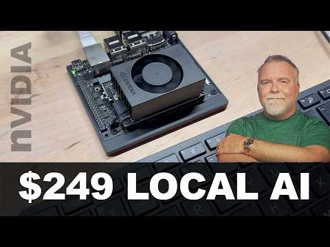
NVIDIA's $249 Secret Weapon for Edge AI - Jetson Orin Nano Super: Driveway Monitor
1M
The NVIDIA Jetson Orin Nano is a compact edge computing device featuring 6 ARM cores and 1024 CUDA cores that enables powerful AI applications like real-time vehicle detection and large language model inference at affordable prices, demonstrating how edge devices can perform sophisticated machine learning tasks locally without cloud dependency.
Click to watch →
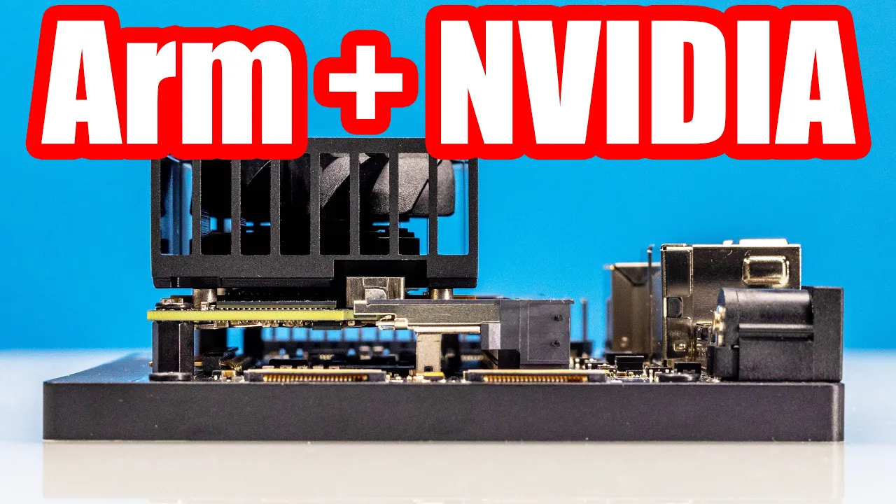
NVIDIA's Low Power AI Dev Platform on Arm
118.7K
NVIDIA's Jetson Orin platform offers two developer kits (Nano and AGX Orin) featuring ARM-based processors with Ampere generation GPUs, delivering 40-275 TOPS of AI performance while maintaining low power consumption (7-60W), making them suitable for edge AI applications and robotics development.
Click to watch →
Core Concept
Core Concept
0:02- 1
Introduces the main topic directly.
- 2
Highlights the speed of the core idea.
- 3
Sets the stage for deeper discussion.
Active Sensing and LiDAR-Based SLAM
While stereo camera mapping with RTAB-Map is a cost-effective and feature-rich visual SLAM solution, it has significant limitations compared to active sensing methods like LiDAR-based SLAM (e.g., Cartographer, LOAM). Passive stereo vision relies heavily on ambient lighting and rich visual textures to extract features. In low-light conditions, glare, or featureless environments like long corridors and uniform walls, visual SLAM often fails due to tracking loss. In contrast, LiDAR emits its own light, providing highly accurate, direct 3D range measurements regardless of lighting or texture. Furthermore, processing high-resolution stereo images for feature extraction and depth estimation is computationally intensive, whereas LiDAR-based approaches offer direct geometric data, reducing CPU load. For critical industrial applications demanding high precision, reliability, and safety, LiDAR remains the industry standard, making it a vital alternative perspective to purely visual mapping approaches.
Basic proficiency in ROS (Robot Operating System) concepts, including nodes, topics, messages, tf transformations, and launch files.
Fundamental understanding of stereo vision, including epipolar geometry, disparity maps, depth estimation, and camera calibration.
Core concepts of SLAM (Simultaneous Localization and Mapping), particularly visual odometry and the role of loop closure detection.
Familiarity with sensor hardware concepts, specifically the difference between global shutter and rolling shutter cameras.
Integrating the generated 3D occupancy grid with the ROS Navigation Stack (Move Base or Nav2) for autonomous path planning and obstacle avoidance.
Advanced optimization of RTAB-Map parameters, such as tuning loop closure heuristics, feature detectors, and memory-management constraints for large-scale environments.
Implementing Visual-Inertial Odometry (VIO) by fusing stereo camera feeds with IMU (Inertial Measurement Unit) data for robust tracking in low-texture scenes.
Deploying and optimizing 3D mapping algorithms on embedded edge computing platforms (e.g., NVIDIA Jetson) for mobile robotics applications.
599 views14likes0:42@alexandergrau887Original Release: 2024-08-09
almost instantaneous n [Music]
Up Next

7:14
Arabic Maqamat Explained: Guitar Tutorial for World Music
@FernandoPerezGuitar
1.6K views•2023-01-13

12:54
Triumph of Orthodoxy Icon: Byzantine Art & History Explained
@BenCallan
2.1K views•2024-08-06

9:49
FastAPI vs Flask vs Django: Choosing the Right Python Web Framework
@TechWithTim
302.5K views•2024-05-26

1:42
Game of Thrones Opening Credits: A Cinematic Analysis
@gameofthrones
46.3M views•2011-04-18
Related Study Plans & Knowledge Roadmaps
Structured learning paths in General & Interdisciplinary Studies
general-studies
Elevator Engineering: History, Physics & Cities
01From Hoists to Safety Brakes: The Dawn of Vertical Lift
02Hydraulic vs. Traction: The Engineering Physics of Elevators
03Modern Speed, Safety, and Algorithms
+ 2 more learning modules
12h5 modules
Explore Roadmap
general-studies
Rubber: Material Science, History & Geopolitics
01Origins of Natural Rubber & Mesoamerican History
02The Chemistry of Natural Rubber & Vulcanization
03The Geopolitics of the Rubber Boom & Colonization
+ 2 more learning modules
12h5 modules
Explore Roadmap
general-studies
Containerization: Evolution, Logistics & Trade
01Ancient Trade & Bulk Cargo: Amphorae to Barrels
02The Industrial Revolution & Cardboard Packaging
03The Containerization Revolution: Malcom McLean
+ 2 more learning modules
12h5 modules
Explore Roadmap
general-studies
Textile Tech: Evolution, Labor & Global Impact
01Pre-Industrial Textiles: Handloom & Cottage Industry
02Mechanization: The Spinning Jenny to the Power Loom
03The Factory System & Global Labor Transformation
+ 2 more learning modules
10h5 modules
Explore Roadmap