

![[4강] Cheng 전자기학 강의 챕터2 (3) 직교 좌표계, 데카르트 좌표계](https://i.ytimg.com/vi/eH0575OjeMQ/maxresdefault.jpg)

![3d Matrix Transformations [Yr1 (Further) Pure Core]](https://i.ytimg.com/vi_webp/pkGXRppWAb0/maxresdefault.webp)

![ปูพื้นฐานการใช้ Python ร่วมกับ NumPy | สำหรับงาน Data Science [FULL COURSE]](https://i.ytimg.com/vi/MDA8SbfdLKA/hqdefault.jpg)





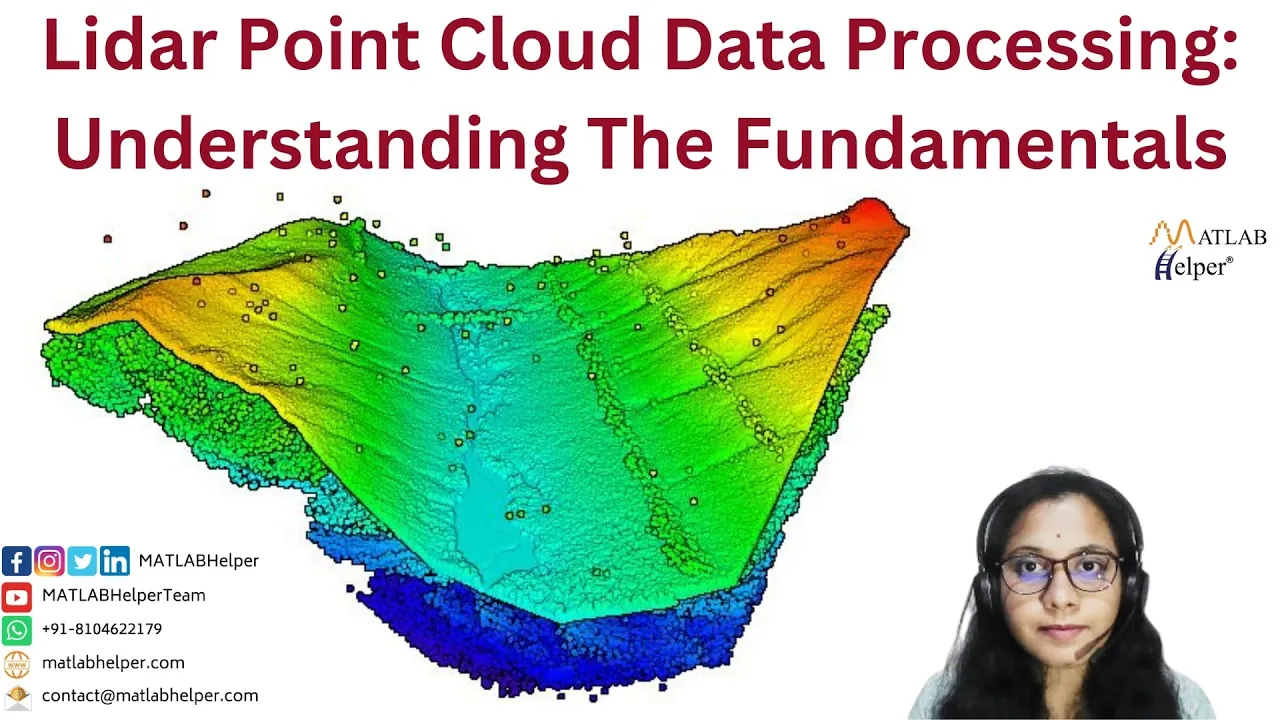










This video provides a comprehensive 99-minute course on 3D point cloud processing, covering essential topics including pre-processing techniques (noise removal using statistical outlier filters and connected component analysis), geometric feature computation (planarity, linearity, verticality, omnivariance), point cloud registration (global registration with RANSAC and local refinement with ICP), unsupervised segmentation methods (region growing, super-voxel approaches), and classification strategies. The course demonstrates practical workflows using CloudCompare and Potree tools, emphasizing automation through Python scripting for handling massive point cloud datasets efficiently.
3D Point Cloud Processing Course: From Noise Removal to Segmentation
Added:Basic linear algebra and 3D coordinate systems, specifically understanding Cartesian coordinates (X, Y, Z), vector operations, and matrix transformations.
Foundational Python programming, including familiarity with data structure manipulation and scientific libraries like NumPy.
An introductory understanding of 3D data acquisition methods, such as LiDAR (Light Detection and Ranging) and photogrammetry.
Basic statistical concepts used in data cleaning, such as standard deviation, mean, and identifying spatial outliers.
Deep learning on 3D data, specifically studying neural network architectures like PointNet, PointNet++, and VoxNet for automated semantic segmentation.
Point cloud registration techniques, such as the Iterative Closest Point (ICP) algorithm, to align and merge multiple 3D scans into a unified model.
Integration of 3D spatial data into WebGIS platforms and custom web viewers using advanced three.js, Cesium, or customized Potree deployments.
Real-world application of point cloud processing in autonomous driving (LiDAR object detection) or environmental forestry (canopy height and biomass estimation).
2.9K views112likes1:39:34Original Release: 2025-11-11
In this 3D point cloud course, we are going to see 3D gion splitting and how to use it. Working with structured data set like oak trees. Moving on to feature computation that makes sense. How to register point cloud together. How to use fun features for your projects. How to leverage clustering and unsupervised segmentation but also how to move toward classification and what comes after that. using this classification in external software where we also have the ability to do measurements do cross-section explore with more precision what we have under our fingers. Moving on to automated workflow to also manage massive point cloud like this one and what are the result of unsupervised segmentation workflow and how you can leverage that for advanced application. Hey friends, today it's a bit special. I want to bring you onto this 3D point cloud course and I will cover this eight topic step by step. It will be a bit of um mix between a hands-on session where I will show you the various stages and also giving you the fundamentals. You will see that this is also based onto a a stream so live event. So you will also get interaction and question about uh 3D machine learning or to set up a labeling data sets and this kind of things. So it will be very very rich. So we'll advise to take your time. I try to condense everything so it will not take you more than two hours to make sure that you can replicate everything and everything is given. I want to issue a small and fair warning that the sound quality is not as good as before because I had some issues and also with the recording but hopefully this does not hinders your uh experience and you get a lot of value of this video that is packed with a lot of tricks, tips and super super condensed.
So leave just down below any comment about what you would like me to work on or what you would like me to better explain and in the meantime have a great time. These are the various processes that we will touch on today. So only the acquisition side we will not target that. That was done yesterday. But essentially you can see that now we have more and more um ways to inject automation and AI into the the capture of the data to have more autonomous capture. So you can see in all the images that essentially robots are acting as a platform on which you have sensors which could be lighter sensor which could be cameras that will allow you to map the environment more or less in an autonomous manner. This is today not the case. Uh mostly we go on site and do the acquisition ourselves but know that there is a lot um in this um domain and for example what you've heard from Muhammad working on slam in robotics. This is one case where you use the slam to guide the trajectory of the robot in order for him to move uh in space. So this is something that is an active research track. Another one is everything linked with pre-processing.
This is usually overlooked but this is the base of any um pipeline and it is especially important.
This is especially important um for establishing something that is robust and that will stand the test of eterogenity. In this case, it's very easy to see that it will be interesting to filter out this point cloud to remove any of the white points that are um noise in this case if we want to only get the structure of the of the of the building. Then after after that we have the registration part. So Eric touched on that uh JP as well with fusing data with different sensor. The first stage is of course taking one sensor and having different perspective and putting that in a unified system. So this is what we see here with the arch. Uh this is something where you have also a lot of research track you can leverage classical methods. I will touch on some of them because they work really well in in some cases in other they may fail and when they fail we push that to more uh advanced methods that usually rely on deep learning strategies.
This is maybe one of my favorite areas segmentation I delinate that really clearly with classification. When I talk about segmentation here it's really having no semantic connotation at all.
It's just mostly linked with clustering.
So having a data set and identifying groups of points or groups of entities that share a similarity criterion. So in that case this is a fully insupervised result uh in a library that was reconstructed with multiv- view um um image. So photoggramometry essentially and you can see that you have a major cluster that I found together. This is mostly a planner based segmentation. And then what is interesting is that you can use directly this as an input to a inference classifier which instead of using every point as input you can use one segment as input. So of course you reduce a lot the the the size of your data set but it means that if your segmentation fail your classification will fail. So this is also something that is worth investigating. Then we'll touch and I will show you a way to do that. I will have to do it from scratch because I actually changed my my hard drive um which was full and I forgot to duplicate everything linked to that. So I will remake everything from scratch.
How to generate um data structure right and in this case a modify nested octry and how you can use so-called potry and you have various um version for that in your day-to-day activities to just bypass any limitation with the size of your data set so that you can explore them quickly.
And finally we have the application layer. So we we pinned down some application. I will try to remind me of them so that when I show the various stages we can touch on that. This is one application that I really like because it shows the power and how crazy it is that surveyor will reconstruct and will take the point cloud and make it as a layer and redraw everything on it when you can automate that. So this is one example where uh we have a lot to uh to do. Okay. So all of these thoughts uh of course were injected a lot in in some papers I I wrote early on uh around the concept of smart point cloud. So essentially trying to see what was done at the time. So we had the point cloud and we had the expert behind the desk right that was extracting a product a deliverable that could be a flow plan a mesh for simulation for a VR project or anything else. um but he was doing that mostly manually or semi-automatically and the idea was to integrate and structure this knowledge in the point cloud itself so that you can use information extraction based on reasonzoning. So at the time I was touching on agents that could handle that and um uh structuring the knowledge in a form that is called an ontology so that the computer could use that directly. Today you can mimic the same um theoretical foundations with u natural language processing and hopefully I can touch on that a bit at the end. So pre-processing this is what we will touch on right now. This is a good example um and this is what I was talking about when I touch on goian splatting. This is the point cloud you get from goian splatting and when you filter out this is something that is a bit cleaner still very hard I think to to use but this is a good example of what uh we should try to do. So just as a reminder yesterday we used um motion splatting to reconstruct splat and I will just show you what we had if you remember with the splat engine this looked pretty pretty nice right whenever you are close to where I was walking so to be close to where I was working I need to see where the camera were okay in the other direction and you can see that it's it's pretty nice right you have the rocks um looks like something you could use whenever you see the visuals now let's investigate the point cloud So I have cloud compare you can export and that's what I did file export splat model as a ply.
Now I will just load that uh in cloud compare and this is what we also did yesterday essentially gion splitting that's just point cloud with a lot a lot of features which holds the spherical harmonics which allows to be leveraged by the rendering engine so that you have a very very smooth and nice visualization experience. um for geometry only it's just that if I go and add a new feature you can see all the features that you have a feature for for reminder it's XYZ there's a geometric feature NX and Y and Z that's the normals RGB that's radiometric features and then you can um extract more features and I will talk about that in in um in a matter of minutes so all that I want to do is just put some color and for that I put DC0 DC1 DC2 Um the normas I don't think they're really useful. So I would not want to have them and okay so this is loading my gosh splatting. So let's work with the point cloud from the goian splatting for the noise removal because it's a great subject as it's super noisy. As you can see here we have something extremely noisy with uh splats floating super far away. So for noise removal the the first strategy is of course go manual. So I take my point cloud. I take the scissors and I will just take some points in the middle. And I drop all the other ones.
[clears throat] This is what more or less I'm left with.
And I will zoom in uh what I have here.
And I will do the same once more. I'm really dropping the point outside. If you are doing any processes, usually you keep them, but for this case, I will drop it. It will be maybe a bit better.
So this is my point cloud, which is super noisy. If I put the let's say the the size of my points bigger, you can see we have a lot of flutters that would be nice to try and remove.
Various strategies happen to work here.
We could for example, so we investigate here. We see that the floaters mainly are isolated. So they have a large distance to the neighbors. This is something that we could use. We could also use features like omnivariance to check on the surfaces. If we have too much variation, we drop the one that are too far away from the local um average or the standard deviation. So usually we play on statistical pointers uh like standard deviation to filter that. So one of them is the statistical outlier filter. You have exactly the same in in in Python that you can do. Essentially for each point you will take a number of neighbors. So in that case if you want to be robust let's say 10 and you want to filter out any point that is above the average distance within the stand plus the standard deviation right so you you have you fit a local model and then you apply this standard deviation multiplier if you want to be less aggressive this will be the case you are less aggressive if you want to be very aggressive this would be the case but in here you will filter out all the points so let's be um like medium less aggressive 10 point and standard deviation of five not to filter out too much noise points hopefully he construct an oak tree uh that he used to filter out the points there after we have the result here.
Already at this stage this was the original. This is the filtered one.
Right now we have a lot of floss and this may be something that is interesting where we could use um a voxal based or or a spatial based filtering technique and for that we may need to move on to um like some kind of preparation because our point cloud is not to scale and it's not rightly oriented. So I go on the top view and I will just rotate my point cloud quickly.
This is just to have something uh that I can work with.
And I will go there and compute an oak tree.
And you will see that now if I draw my oak tree, this is what I have. And I can select it and go deeper.
Yes. Until I have a a specific numbers that allows me to have discontinuities, which will allow me to filter out really the discontinuous floating elements. So I could even go up until the eighth which in this case would maybe work.
Okay. So let me do that. I take my point cloud and I do a filtering based on connected component level eight and I want to keep only >> [clears throat] >> um segments. So clusters with more than a thousand point. Okay. And this means that now I'm left with there's uh four clusters. This three I think I can remove them for now and work only with that. So this is the result of my point cloud after filtering.
Is it good enough or not? Hard to say at this stage. We still have some uh some noise.
But it's better than the original.
So now maybe we could use the feature technique to go beyond only what we did.
And for that you can go on to edit [clears throat] um tools sorry sandbox no others comput geometric features. So again this is something that we do in python. This is just for the sake of a presentation to make sure everyone gets what we are doing and visualize that. Essentially we will use a local neighborhood radius. So this is based on a fast marching tree.
So if I reset that it does not change at this stage. uh you can move that to any number that you think makes sense. This is highly impacting what your feature will represent. A very tiny local neighborhood will mean that you really look at a super tiny local region whereas if you take a large neighborhood um essentially you have more global feature and you have some kind of multiscales approach where you compute a feature at multiple scale in order to then do some kind of difference to really understand if you have a change that happen only locally or globally.
And that's another type of features that is derived on previous features. And what you can see here is that most of these features are based on um on values and igon vectors. So principle component analysis. So derivative of the the local areas. What is interesting at this stage is maybe for me to show entropy plarity linearity surface variation and only variance.
I will let him compute that because in some cases it can take quite a lot of time and this is why it's always important to do some kind of pre-processing stages to make sure that you remove unwanted artifacts.
This is here the results of our feature extraction and you can see that we have okay so I will open that a bit more activist surface variation. So if I take omnivariance this is what I get.
We have uh all the points in gray are outside the range that is here visible.
So they already filtered out. This is already super aggressive as you can see.
But it will leave only points that looks relevant on the geometric side. But it may be really aggressive if I were to use that. Now we have entropy entropy.
This is um what you have. It's a bit less aggressive. So this may be better in this case. This is mostly the point at the edges of elements that get filtered out. You have plarity. So of course nothing is really planner here.
The if I were to check what is planner, you can go on parameter and not show that. This is what you get.
Again, my radius choice maybe not the best here. It's maybe a bit too tiny.
The linearity uh same thing. Let's check that.
So it's still better and suffer variation is really aggressive. So if I do that, we have a lot of points going away, right?
And omnivarians. How was that? Um this is not entirely bad. So let me work with that. So what I do is actually I will take my point cloud. I will activate a specific scalar field that I want to use to filter out. So it's a it's a thresholding. We are actually segmenting the point cloud based on one feature. So it's thresholding. I'm doing that manually. But imagine that if you code essentially you compute your feature and after that you establish a threshold that makes sense. Here I use my um the visual qualitative analysis to define the threshold. But in case you want to have something data driven, you can extract that from the data itself.
So you will sample something in a specific uh planer region in a specific spherical region extract what kind of feature number you have and you start to guide the threshold mechanism and here I just do that with the GUI. So it will be edit scala field filter by value and in here because it's outside the range I would just export everything uh that is within the range and this is what I get.
Now, the RGB is really not the best in that case, but it still uh viable in some aspects. Just that the black points are are um maybe hindering a bit the process.
But yeah, I think that would be fine.
For the next stages, what I can do is reapply a filter to remove all the the noisy points. So, let me do that. This time I would take only five or six neighbors and I will be really aggressive.
And normally I should get something cleaner. So let's see.
Yeah, this is a bit cleaner. And I will delete the floating point again.
Okay.
And this is good. And the rest I drop it. So we have one main element which is much cleaner than uh the one at the beginning. Yeah. Which was rotated and had a lot of stuff. So this is our new point cloud. Again this is extreme what I did because the question plotting is extremely noisy but this will allow us to monitor a bit better what we are dealing with. One last thing that I can do maybe is I will duplicate my point cloud not to make any mistake and I want to show you a little trick to improve the qualitative visualization aspect. In this case, I mentioned this is from uh this is not true RGB. This color are normally super imposed with the goian splat spherical harmonics. This is why this looks really saturated and we have blacks and stuff but normally uh this is how it should look like whenever you use the spherical harmonics. This is something I did not do but you can do that of course. Um, now if I wanted to improve that a bit without doing a heavy process, you can use the PCV uh, which is essentially doing some kind of occlusion test and creating a scala field that you can then superimpose on your colors. So, let's try that with a 1,024 resolution so that it doesn't take too long. It's sending rays from above. Oh, it's so good that I um actually um duplicate it because I think when I did the rotation, I put it upside down. So everything may not be uh as I want that to be. Yeah, this is what I meant. So it it sends the ray from above in uh all the spherical direction to create a scalar field to mimic a bit uh where you have something black and something which is not black. The problem is because my point cloud is upside down. This is how it happens to to result in. So I will delete that. Take again my point cloud and just do a rotation around the x-axis. This is fine to put it uh in the other direction. I will clone it again and do my occlusion only northern hemisphere plus and press okay. And this should bring something which is a bit better in our case.
Just checking if there is anything in the chat. Okay. Okay. So I need to order the point cloud in takes a few hours.
Okay. So I may do that and we may have that for the second part on threedimensional.
Nice. So this is what we get. And look it really I I like this kind of visualization especially for such natural point cloud. But you can see also very clearly how noisy the geometry is uh with the with the goshion splitting. When when you look there it looks all smooth and nice. But if you if you take a measurements the underlying and here it's filtered out is really not as smooth. But again um this is also full of grass. So this is also why you still can use that for doing counts and various measures that don't need specific metric accuracy but more um exhaustivity accuracy. So if I were to to count the the the rock mass here maybe that would be enough. And this is something that we can use thereafter. So what I will do here now that I have that is try to combine uh colors enhance with intensities. And normally it will use my scala field to enhance the colors. Let's check that we are between zero and one.
So this is good. And the intensity field is illuminance PCV. And I press okay. Um yeah. So, this is not entirely bad, but because of the saturation of my colors, we see weird elements, blue and red on the rocks, but it's still better than u just the colors themselves. This is something that we could filter out after. We could increase this as well.
So, if I were to enhance that one more time, maybe that will um make that a bit better. Let's check. No, does not change.
Okay, so we'll leave it like this at this stage. and uh visualize that afterwards. So what I do is I take my point cloud like this file save and I will save that um as a last file and for that let's go onto the boot camp chapter 3 and you will have the data set then uh filtered point cloud and I will keep the las for now 1.2 two custom scale. Okay. Uh we leave it like this. Use minimum bounding box center.
Okay. And do I want extra field for now?
Not. I will just keep the the parameter as they are. Okay. So now back to our um process chain. This is the filtering that we did except we already did some kind of formatting for the registration part. So let's maybe explain a bit on the registration side what we want here.
In the case that you have not aligned point cloud, you want to bring them and align them. So I could do that. Do I have some point clouds? Imagine you want to bring these two um point cloud into the same frame of reference. They are normally they are the same but we could like play with them. Put on some gian noise uh add some specific remove some points and such. In this case, it will be interesting because we can monitor if it's uh like perfectly fitting the same registration. You can do that also within Python just to show you what's happening. So there is two stages here.
Um there is the global registration challenge and there is the local registration problem. The first stage is to try to push that and bring that in this frame of reference and the second stage is to try to fine-tune the alignment so that you have as a minimal um distance between both shape as possible. And this is what is done whenever you go onto slam mechanism.
Each lighter pulse will bring you a point cloud and you have a time stamp t where you move with a small displacement and then you want to merge that with the previous one and so on. So what is done here usually is the global stage will leverage renac to find point that belongs to mostly the planet surface and you will also use the bounding box to align center and use renac to bring them all on top of one another and also uh you may you may use also a bit of a rotation around that to find a global registration automatically. And the second stage is then to use um a local registration mechanism like ICP iterative closest point to try to really uh bring the point clouds together much more tightly. So let me showcase another way with points uh that will be the same in both point clouds. So the local and the global. So this is the local one. Let me check in both case. So this is the good one. So tools edit color. I will put that in blue. And this is the one that we want to change. So you can select both of them. And normally you have a way to um like push them together which is here aligning two clouds by picking at least four equivalent pair of points.
Try to take those points in areas that are easy to pick for you. Um and here essentially you have a square mechanism that will give you the more point you have uh the better the the fit will be.
So let me align quickly select the to be aligned entities. So uh select all global and local. Okay.
Okay. No sorry I just take them again and I align. What is to be align? This is the global to-do registration target.
Okay. So this is the to be align and this is the reference. So we are good.
Now what I do is I will go for example um I would take five points. So one here one at the entrance. So I will go there.
I will take maybe the first one will be at the entrance. The second one here in the corner. The third one will be down in the tree. So we have three there.
Okay. We have a pole here. Interesting.
So I would put one on the pawn A3 and uh one here. Okay, A4. You have to do exactly the same thing on the other point cloud.
So uh the first one was the entrance.
Where did I took it? Oops. Sorry.
First one was around here. I think I'm getting very rough. The second one was there. The third one was on the tree.
The fourth one was on the pole. And the final one was uh here or no, it was done. So you can remove the final one.
No, was it? And what you can see is already the error. So let me add the person.
So uh you can see the error for each of the the points. So 1 2 0 0. The problem is I know in this case we are to scale.
So we have one meta difference 2 to22.
So we have a problem in the pointing of the R0 and R1. So let me check where they were.
Yes. And here.
Yeah. Okay. There they are bit. Okay. So this one this is normal. So the R1 is not good. So I will delete it as well.
[clears throat] And you see that the fit is much better because we had an error in my point. So let's keep this fit and put a line and validate. And you can see we have the transformation matrix that we could use and we have the final root mean square error which is around 20 cm. So this is a high but normally if you are below a certain threshold you can be fine for the next stage of iterative alignment.
So I guess here it will be fine. So let me press okay.
And this is what we have after this first stage. So we have a problem with the ground. Um but yeah this is our global registration. This is what you can expect to have whenever you do that automatically.
The second stage is to do the same but instead of picking pairs we will uh finally register point cloud with ICP.
So the tob line is the global and the reference is the local. You can define a number of iteration else you have a a stop criterion that is based by uh the root mean square error. Right? So this we will keep that in some cases where you have like various perspective with a change in scale you can add that of course this add another parameter to estimate by the algorithm so it's it will be less accurate or it will take longer and we we can use normals also to guide in order to uh fix the rotation around the z-axis.
Here in the research tab you can give how many points maximum you want to use.
Um, so that's a sampling limit. This is for the algorithm to be efficient. If you if you just care about exhaustivity and accuracy, you should move that up a lot, but it will take much longer. And you can also ask what kind of rotation and translation you want to adjust. In this case, I want to keep it and leave him the choice to change each parameter.
It's a rotation translation, but not scale. So, six parameters. And you can also ask him to enable any point that is too far away by clicking here. So let's just keep it this way. I think it's fine. And at the end you see that it aligns.
Yeah. Okay. Let's check what's happening. But [snorts] he says essentially we have uh an RMS that is worse. So I think we did something that is not good. Theoretical overlap 100.
I know. Okay.
It's okay. So it's because it's a perfect match. This is uh why cloud compare cannot handle where the visualization. That's interesting. I've never seen that before. Okay. So uh this is a perfect case. This never happens.
But here it's because we have exactly the same points.
Still it allows to to check what you can get from um this mechanism of global to local registration.
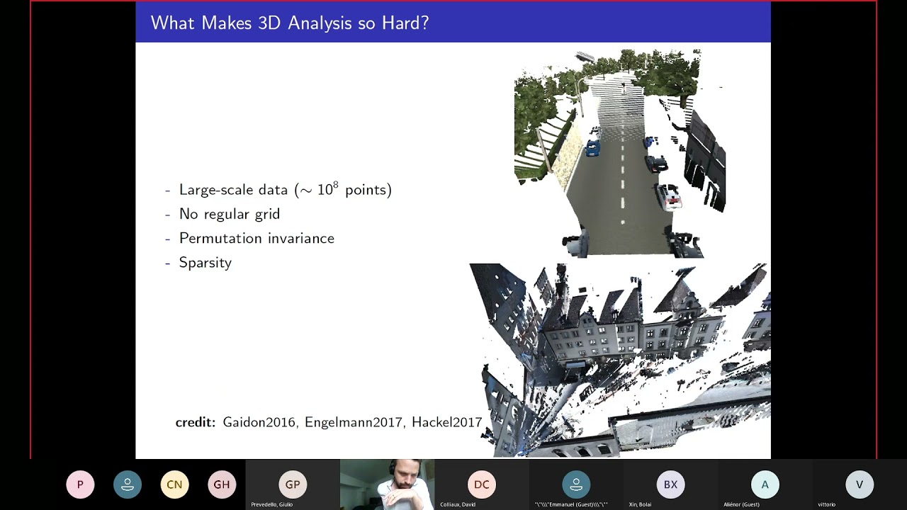
Now registration we did that. Let's move on to um segmentation. And this is where I think it's important to speak about features and also various way that we can do segmentation. So with cloud compare I cannot show you all the way to segments but I will speak also about others that are super interesting and maybe maybe maybe I can go through that before going on to the the cloud compass side of things. Um so there's a some example of segmentation that can be useful for you. Above you see that what we do is what is called difference of normals. So I spoke about the nature of features and how you can play with scale when you compute them. What is happening above is exactly what I did. So you have this street scale level point cloud and I computed normals. So to compute normals you do a principal component analysis and then you take the igon value with the so the igon vectors with the lowest igon value and this is the third component that will point up of a local surface area. So essentially what that means is that you have a point you take a um a radius around it or you take a k nearest neighbors you compute your igon values and vector and you get your normal then you change your radius to something bigger and you compute your normals and then you do a difference between uh the the big one the small one and you divide that by the the value of your deviation in both case and you get the difference of normal which is a measure that will hint at where you have a change in the normal direction based on the radius that you have that will highlight a lot the edges much better than taking a single uh normal and also it will be much more distinctive and robust to any um like local global change. So this is what is done and then after we do a magnitude result and you can see uh what you get and from that you can do a distant clustering and this in this case you will get some windows uh the the side of the buildings and things like this. So this is one way to leverage that and maybe I can show you how you can do that in cloud compare.
This is feasible. Another example is whenever you have tightly bounded point cloud like this one you have the capacity to still use features to extract special characteristics compute facets and do the car mean based facet refinement and then region growing. So this is also a process that I like because it shows you that you don't go directly to the optimal case. you need to go through an intermediate step of having segments that are a bit bigger than points and that are used then through a region growing mechanism. I will speak about that a bit later. This is another example where you get the results that you see here by going onto again um a segmentation that will compute some kind of groups that are really not making a lot of sense for taking them as an individual component.
But then you use that with growing mechanism to obtain what you have on the left. So this is called super voxal, super pixel or super point mechanism. So creating this kind of groups of elements on a local subset that will help you drive advanced segmentation mechanism.
This is another example uh for [clears throat] indoor data by Stanford.
And in here essentially this is the labeling process that is illustrated here before moving on to pushing a canonical space that is then used to train point initially. So you can see that uh segmentation does not necessarily apply only to geometry but you can also have that to spaces. This is very important to understand that sometime what you are searching for is not a geometry component but more a space aware connective uh um segmentation or segregation. Two concept to have in mind are over and under segmentation. So over segmentation is when you create too many segments and it's actually a burden on the computational capacities because you will not be able to go on to the result that you initially wanted. And the second stage is under segmentation. And this one is super problematic.
Essentially this is when you have a region that bleed over multiple object that you want to obtain. So this could be having a segment uh on an edge that bleeds over two facets. If you want the facade independently, this will be problematic. So this is what should be monitor under segmentation. This is the metric that should really be monitored.
On the cluster extraction side, this is very very powerful. This is what we did with the connected component algorithm.
But uh essentially this does cluster extraction. This is super powerful. It means that you need discontinuities discontinuities in your point cloud or your feature space and this is something that is not easily uh feasible in some cases especially for land um vegetation and uh natural elements. This is something that is not super easy. The region growing algorithm this one is is um is given to you in the 3D segment OS with an advanced version. This one is super super useful in a lot of cases on 3D data sets where you can essentially take as seeds uh you take some points or some cluster and you will grow region based on a on on checking a feature. In this case you grow a region based on the normal. Whenever you have the normal that will change higher than the threshold that you delineated then you will have um a new region that is created. And you can also be smart about the decision at which point you start with for growing a region like starting in planner region.
This is something that is um usually smart and also you can adapt the threshold based on the data and have something that is not fixed for all point but knowing that if you are in a curvature intensive area maybe the threshold will be a bit higher. This is something I will speak a bit about later because you have ways to have this mechanism work without any knowledge injection. So fully insupervised, right? So for segmentation, let's uh keep this one maybe because it's a a good a good example.
We have everything here that is tight together. If we want to segment that into various features, I think we should use features that look at if an element is planer or not. So for that, you know the drill. Now other comput geometric features, the radius, I will put it a bit higher in this case. And I want planerity, verticality, linearity, this is okay. and omnivarian to check if we have points that um in some certain areas don't follow something which is usually flat or you have a lot of deviation between points.
Okay. So this is the extract from what we have. This is using verticality. So you can see that we could use verticality for example to uh filter out the ground. But before going there let's check the other features. So omnivariance I thought that will help for the trees. It does not. So we may need to to use something else. We have branches but that's all. Maybe linearity will be useful for the branches. Yeah.
So linearity you see that you you have all the linear feature really nicely taken and that could be the seat then to grow some kind of clusters for the trees. What else do we have surface variation? So this can be useful for the elements that is grassy on the ground but also to detect whenever you have change uh in the in the normal direction and this is what you have highlighted here and verticality is good to like define the ground from the rest. So I can start with that. If I were to filter that out I would do edit scale field filter by value and I would split not here. I would take my point like this.
The problem is I have floaters here. Uh so I would need after to to delineate them. So edit scatter field filter by value split and I will call that segmentation.
Okay. So this is what I can work with for um the ground.
As you can see, we have all the floaters here that are a bit annoying at this stage, but are easily taken out by just going on the side. You could also use edit um to scala field convert export uh coordinate to scala field and only the Z for example. And this will allow us to filter out based on the Z value. So I will not be super aggressive, but I will take that. Again I'm doing all of that uh visually but you can see if we take the histogram here just to show you this is what you have. So this is also very very handy and powerful in this case um you can detect the peak right and this would be a hint to segment elements around that fit a goion and that will be the ground. So you can directly see the goshion here. If I were to fit the goian it will have a slight um slide because of here all the various other elements.
So what I can do is stop at the value 3.14. We have the 68% of the of the point which is linked with the gion right the sigma value. So I could take that 3.14 to filter out my point cloud. And this is done like this filter by value 3.14 and split. Okay. So I will just seeds.
This goes in seats. So now we have that this is mostly the ground that can be refined and this is the remaining elements um which could be further extracted I guess with other strategies but in this case I think you really need to have a a plan based detection to get all the elements on on the facads and all. So here I will go with region growing or planner planner face detection. Maybe I can do something around it with Python for that. Just right after because with cloud compare I may not be able to to show you the extent of what we can do. Just let me try something. We see that we have something that is mostly planner right.
So we can use shape detection and use that as a way to guide our segmentation.
So that could be renac. Uh if I go there you have the possibility to use renac.
We will take only the planner um elements and have 500 point as a support. Keep all the leftover points in a new point cloud and do the square fitting on shape. I don't want to simplify the shape. And for now I will set random color but else you you don't do that. Max normal deviation 25°. Okay.
Sampling resolution uh the distance between neighboring point in the data I will put it at uh yeah 0.5 is okay.
and the max distance to the primitive 0.2. So 20 cm that's high but again I don't know the the resolution and the precision of this point cloud. So let's try it this way.
Okay. And yeah as you can see it's not entirely bad right we have found most of the facads in our point clouds as segments and normally he save the leftover points here. So I just take all of them toggle and this is what is left to activate the normals. So this is kept as noise but again you can have a refinement step that will take a seed every time your region and grow a bit to make sure that all the remaining elements get taken out.
So we could continue in this fashion until we have everything in a segment and then move on to the next stage which is uh classification.
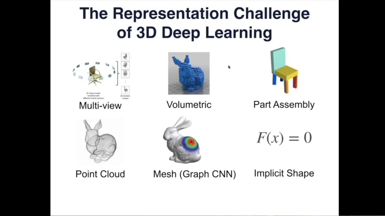
So classification what I mean by that this is a a meta category that host classification task, semantic segmentation task, instance segmentation task, a panoptic segmentation task, object detection task. Essentially everything falls within this umbrella.
This is not the case with 2D. Uh with 2D a classification task is really you have one element which is usually an image and this image will be tagged with a class. Right here, classification has all of that under the umbrella except whenever you deal with object detection.
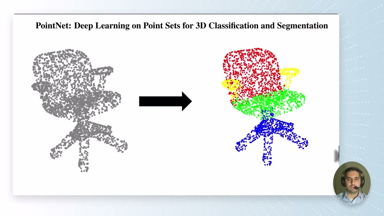
If you pass in an entire point cloud through your algorithm, then you can add a label to the entire point cloud which is then a label classification task. You also have things called part segmentation where you have an object and you want to delineate subobject. So the chair is one object and you want to go beyond that and have the legs, the back rest, the seats and things like this. So for the classification as I mentioned before we could use that as a guide. So uh toggle I will just show you also a way to quickly select the various plane. Um so select children by type type plane. Okay. And then I think you can I know select chill my typo name I will just delete them for now and all this point cloud I will bring them in the same one. Yes. And remove the normous. This is our main building and this is the rest. And this is the ground and this is the remaining element. So I have to put the ground there and I have to put the remaining elements. So this is what we have.
So we should be normally working with that. But again what you can do is increase uh the threshold of the renac maybe to keep that. And I will still work around with trees. So to work around with trees I can use in this case I think a connected component being aggressive and normally you don't want to drop any point. This is just to have something a bit clearer. You don't want to colorize it. This is again just to showcase what we can obtain. So this is an over segmentation but then this could be the base to grow from um in this case and it's much easier to work with um like we have the main trees and you can grow taking this big region and attaching all the other elements based on that. So usually especially for forestry terrestrial laser scanner what you have is a cut graph cut approach where after that you construct a graph and you compute the connectivity of components in your graph that is guided by some kind of algorithms to define and delinate this major segments. So this was just to show you what you could obtain. What I will do now um because we are a bit limited with the time is I will do the same but be less aggressive.
So I would keep eight and 10 and you see that we have major segments uh obtain essentially I would just check the major segments.
Okay. Okay. And all the rest.
Yeah. I cannot hear guide it too much on the size of the segments. This is a bit annoying me. But do I have for example this tree here? Yeah, this is a tree. We have the tree pretty nicely taken here. It's maybe a bit big, but still it's a tree, so that's fine.
And all the other remaining elements are dropped. And here we have also windows.
As you can see, we have all the windows independently taken, which can be useful.
Um and here we have the entrance as well taken with a bit of trees.
The pole also is taken here alone.
So that's can be a good base. So the next stage from that will be to just work um again you should not do that manually because else it takes quite a lot of time except if you are constituting a label data set in which case you have to go through that. So what I will do uh if I were to doing that is I will select my various trees for example and put them. Okay. So you first need to have to constitute two groups. So leftover and group. So in here I will take my trees like that and put them here that I will call tree.
And every time I put them here I deactivate them.
Um, okay. Tree. Tree.
This is just to see a bit clearer. This is also a tree.
All right. All of that is also a tree normally.
This is a tree. This is a tree.
Now I will create a new group ball that I will put in between.
For some reason, I cannot, but that's okay.
This is a pole. And we had another one, I think.
Yeah, there a bit over segmented. That's also P. And that's also B.
I'm uh okay. Yeah, that would be the stairs. But let me then bring in the uh group of show the tree and show that would be the building ground and uh I would call that uh noise even if it's not really noise. This is just to show you the next stage. Now we have the building, the ground, the noise. I put that here. We have all the trees and the poles. So what you do is you take the trees all in and you merge them and you keep the new uh original cloud index. This is for the instancing. Same thing for the balls.
So I put that here for the balls. I bring that in. And yes, of course, here I have a problem of uh over segmentation. So the instance is not really the pole, but that's fine for the demonstration.
Now this is our final point cloud. What I will do now is make sure that the building we have an original cloud index. This is if you want the facets, right? So we have a facade de composition which is fine. For the ground we have only one element and for the noise also one element. For the trees, we have multiple elements. So, we have original plot index. I will just go there. Um, Scala field rename instances the building I will call that then facad. And the original cloud index you rename that uh as instances ground noise trees we have instances and poles. Same thing. Edit scatter field rename instances. Okay. So the next stage is I will just duplicate all of that and I'm taking them and merging that uh and I I generate this calf. This is why I renamed. Now normally we should have everything in a single class. So the last stage that I can do is instead of having that called um um original cloud index I rename it and I call it classification and this is my classified point cloud in uh trees building ground and poles. So you can see that it's absolutely not perfect but it's a strong pace for already getting something that you could use to classify or to extract specific features. This was done in under 15 minutes manually but you can automate that and maybe this is something that can I can show. Uh but before showing that we can move I just check if there are any questions. No, I think we're good. We can move on to the final stage on this um uh part which is structuration. And what I will be doing with structuration is creating um creating something. This is what we did. We gathered the point cloud. We studied the characteristic. We generated features. We use them to create labels.
Um this is possible to prepare the data set for the next stage. And now we will create a visual tour for the point cloud analysis. So this will be also our application. This allows me to speak a bit about the standard format just to make sure that this is clear because I remember yesterday I don't think I touched on that. You have three main categories. You have as key file format which is very useful if you want to stand the test of time because you you can open that without external software.
Normally each operating systems come with a way to read ASKI file which is essentially a list of um elements that is uh not binary. So you have XYZ, TXT, OBJ are the kind of ASKI file that you will get for the binary part. This is something that is much better if you look for optimization on and compression. The problem is you are usually linked to having some kind of library or some kind of software that can create and read this kind of elements. So this often happen that you have a software that makes super cool stuff 5 years down the line they stop because they are not profitable or something and you are stuck because you did not convert that into format widely used. We have hybrid format. PLY is one case where you have a little bit usually in the header that is plain ASKI which allows you to read the file and then you have a part which is binary that just ask you to have some elements to read that more efficiently. So now before going on to the common line uh interface let us go and install or show you a way to handle massive point cloud. As I mentioned I I deleted that from my hard drive so I need to to do that. So you have a tool which is called um poetry which was developed um in Vienn that's a spin-off as a scanopy project and Marcus shoots which is a bright computer graphics computer vision engineer made a version for the web with webgl so that's Marcus and you have various distribution you have one which is potri which is on the web which needs from you a server this is not so hard to do but this is not entirely straightforward and you have another one which is called potri desktop which essentially rely on electron to create a distribution of this web version for the desktop. So, it's easy to just get it. You go there, at least for Windows, uh you download the potry desktop, we'll download it. Uh yes, and I will just install it um on my hard drive. So, I go to software, I push it here. The thing is you have nothing normally to install. You extract it to potry.
H you you are not seeing. Sorry. Um [clears throat] this is what I have potry 1.8. I will just rename it.
Okay. This is what you have in it. Um actually the X file is the potry desktop.bat. So what you can do is uh create a shortcut and on the desktop you can just rename that.
Uh okay viewerware and put another icon if you don't like that. This is me being crazy, but I think Okay. Yeah. And the icon. Change the icon.
Okay. Um something. Yeah. This one. Okay.
So, this is our point cloud viewer. I had it before, but as I mentioned, it's not uh anymore working. And it open a portry instance, which is local um and you don't need any dependencies on the web. So now what he did is also nice is that he integrated the conversion. So which is called potri converter which allows you to go from any like last file format to the modified nested octry. And if I were to take what we extracted before which should be now uh here. So boot camp chap 3 then the filter point cloud if you remember in l file format.
If I drag and drop it here you can convert it. I suggest to use the 2.0 because you have less files, okay? But it's not compressed at this stage and you start the conversion. Uh you should not take too long. So this is done once and after the file is is accessible directly. So now you have your point cloud uh where you can move around in it uh directly which is pretty pretty nice. So, okay, this one turns out not to be as good as what we have on the go uh splitting side, but it allows to check for any inconsistencies uh that you may have. So, you see that is super noisy, super super noisy.
Nevertheless, we have some interesting elements there. What I can show you maybe is on a bigger data set. So now in there you have your point cloud that is there and you can show other uh information.
If you had classification you could show classification intensity and for the classification maybe this is something that we can try is exporting all data set with the new classification file save. This is a tiny one right but still chapter 3 facads.lass plus save. Save.
And all that I have to do is drag and drop in the viewer.
And this is what we have now. This is the classification field active. So this is a great way to share things uh with your collaborator as well, right?
Without moving too much out of your comfort zone. You have also a lot of tools u like measurements. So this is a measurement that I can take.
Right. Uh 16 mas you have possibilities to create uh section cuts and sections.
So here this is also interesting. If I were to do that and now show I have my cut we don't see it really but if I just show only inside method. Um where is it?
Did I created it? Yeah. Normally this should be my profile. You can show the 2D profile. Yes, but I want to show only inside. You have your cut that is there and you can adjust it. So if I take my profile, I can have a larger width to play around with and you can show the 2D profile which is super handy in this case. So let me open because you can have all the characteristic on the left as you can see and this is really really nice. So you have the trees and you can extract some kind of element and in here you also have the possibility to extract this profile only in LA file format. So that means that you are not stuck to only working with something in read only. You can extract element and rework them in cloud compare. So, for example, if I wanted to work around with that, I could do that. Um, extract the profile.
And now, if I go there, I have my profile apply.
Um, yes. Okay. I guess I shifted it. But this is the profile then that you have.
So, you have the in and out.
You have a lot of cool stuff to do. One thing that I want to show you is the massive point cloud, of course. So that I have on my data point clouds. Um what I can show you. Yeah. Okay. So for example, this is a huge point cloud.
Um let me restart to make sure that we have something that you can replicate easily.
So I open my viewer and this is a huge point cloud that is 100 uh giga like 120 GB. It's converted. that just drag and drop it and in less than a second you have the entire city that you can uh navigate and of course this is where you could move around extract some specific features uh make some kind of analysis at scale.
So this is really interesting you can also load in all the point cloud um and like combine some kind of elements. So let's go on intensity gradient monitor the height uh quickly. So if I were to put elevation This is then easy because you can actually work with normally the range right to color elements. So this is also cool. It's exactly the same filtering capabilities that we saw and classification if it has yeah you can then show what is the ground and what is not the ground and work around with that.
Also the return numbers everything linked with your um point cloud. So if you did not know you could do that. I think this is a a really super interesting tool.
Working with classification also allows you to like do some projects um pretty efficiently. So in here we have that in high vegetation for some reason no vegetation. So you could compute how much area you have taken out by like u this little fontain I guess. Yeah.
You just go on to the tools and here if I do that very quickly you see uh what you have as a fun fact this is actually um with open data today especially this is something that I use almost every day whenever I need to check out if a project is suitable or not for the legislation in France. Uh for example, if you want to create a pool in your garden, you can use point clouds uh with open data like put here if that was a pool, you know, more or less the size like a nice pool 10 m by four, right? And you could check if it's on um parel, you could check if this is in the area fitting to the regulation, if you are load or not. you could check out if the construction that you have has a height uh which is suitable for the local urbanism plan. So there are a lot of things that you can do directly and leveraging also the classification is something that is very very uh powerful especially for example Eric you mentioned in Norway the capacity to have very nice data set in France you also have a nice data set which is already classified and this allows you to filter out only point on the building to be able to leverage that for uh getting this uh like how much building you have on on specific area or things like this.
So this is something that I really wanted to show you that is really useful. Now maybe I can talk a bit about how you can bring that all in with Python and um how should I do that is spinning off maybe a mini cond first. If you remember from yesterday cond I will just open that and zoom in cond list. This is all that we have.
Yesterday we had the boot camp. So I could go back onto this on the activate boot camp and um normally I should be good to go here. Um we have mattplot lip we have all the libraries uh installed normally. So that should be good to go and we used spider yesterday. So I will just spin it off and we can move around from there. So just looking at the chat if there is something um there is something that I've missed.
What about lass and laz?
Yeah that's good. Lass and lass works the same. Uh if you mean the difference between last and lass is compressed and lass is not compressed. So they use a it's last zip. So they use a zip comp compression on it whereas the last they they don't. But both works.
Um the thing is of course if you have a compression mechanism you need to have a decompression mechanism. So opening a last is is longer than opening your last file.
[clears throat] So that was what we did yesterday. Let me uh create a new um a new script to spin off cloud compare with various processes. So the first thing that I want to do is maybe um save that save as chapter two. Um I will call that pip line or uh automation point cloud py save set console working directory um in here. So this is not tested on Windows 11 and Mac OS. So this is just that and um I can import um three libraries for now. So subprocesses this is what I mean. This will allow us to uh to work with changing specific software. So one importing libraries and as I mentioned yesterday I like to work with best cells because it allows me to move step by step. So the first thing that we will do then is uh also maybe import uh macro li and we will give way to operation one operation at least or operations um that we will call later on.
So that will be our variable of operation that we want to do. Okay. So essentially we will call a subprocess and this is how uh it goes.
So let me just copy what I had made before and modify it.
So we just use subprocess and we will call a subprocess which in this case is cloud compare. You see that I have to pass my uh path. So if I open here this is where cloud compare is installed cloud compare.exe. Okay. So O is for opening. Uh maybe I can show you that with cloud compare. If you if you want to use the sub processes you need common line access. So cloud compare has this compare it's called CLI and we talked yesterday about reality capture the same it has CLI so you can use that and with meshroom also. So you can do that for the um acquisition part as well. So O is for opening basically in the common line. This is where you have all the available options. So this is for the latest version for mine. Maybe it's bit different but it should not be too different. And what you can do is just chain various commands. You have some example I guess at the end. Yes. So if you do cloud compare open global shift auto my large coordinates. This will um open and and switch and do spatial subsampling and export your data. So you have some kind of example cloud to cloud distance uh cycling over files. You have also some batch to do bundler mesh conversion. So these are the small example here. We could chain the various processes that we had. So the first thing is we should open a sample. So in my case I should have a a sample data but we will take the one from the chapter chapter 3 [clears throat] which was um chapter 3. Um so the facad is already processed but maybe the one that we load it will be nice right so that was um this one and I will put that into a data folder and I will call that sample but that's a ply so let me transform that into aski for now oh but no uh cloud compare can open py without problem so we don't even have to do that so you can also use that for E operations.
Ah, it reopens uh CL compare which is fine. Just let me bring all of that in here and close that.
Okay, so we have in data sample.pl. So this means that you can do that export format l save cloud uh file and we will do results.
Right click uh copy as path. It should be something. Yeah. And I will just do that.
Uh the problem is I have um I have a little um space. So I will remove that if I can.
Yes.
Okay. So let me try that.
I think we have an issue because of that.
And this I comment for now. So let me import that execute and just check quickly if everything is working.
Uh DPCD sample does not exist. Yeah, this is my mistake because it's um here.
Okay. And I just need to do that. So now if I do Why does he have a heart? Did I put the heart somewhere? So I guess so. Someone I heard someone needs to join.
Okay.
Okay.
OpenG. Ah, this may be problematic to work on with a a space. This may be the problem. So, I may need to move that out.
Just let me try by switching to slash instead of backslashes.
Two file name, but they are one cloud.
So the backslash is fixed my problem. Uh the last thing that I need to do make sure that I open one file. So call open g. So essentially just to show you this is a list that I pass. This is how my list look like. We have uh the path to my program. We have open and every time with the process it will just in between add a space. This is fine. My drive course was boot camp chapter 3 data sample. I just need to check if that's the right path. Chapter 3 data sample.py.
So this is good. [gasps] Export format l save clouds file. But because I have only one file, this is maybe why uh it's not happy.
I may uh be able to actually bypass that. So take that push that here comment and um yeah just set to last change cloud put for not finish and that's the safe class that is not uh happy two file name but there are one cloud so I just need to make sure that I use safe cloud the right Okay, which is here all at once.
Okay, file.xxxx.
So, I would just put safe clouds without my little um this is if I had more not entirely sure here. Let's check my draft chapter results. Okay, I understand why now.
file. I forgot to put results.
Still not save Cloud. Okay. Check console drive boot count chapter 3 B results.lass.
So it did save it. But where save finished? I think he is not happy with me giving the path.
So if I were to do that, I guess it will work. Problem is maybe you save it in the in the wrong folder. So let me call it. Yeah. Uh save clouds.
So if I go to data, okay, it's saved in the original directory which is fine uh in the layers. So things are working through Python [clears throat] now.
what uh we can do is just define the base information for simplicity and then move around from that. So let's do that.
Um we give the path we give the data path in our case then this uh we can give the output path. So in our case it will be this results uh the name export and file opening is a ply and I think from there we can do some kind of um e operation. So this is how you would write something. So for the import part you see that you can create a variable you pass in the path you don't want to bring in the time stamp that we had at the end you want to save it uh and you open the file path and for the export format the file output and save clouds so file o is pl that's why we can put bin to have something in the format of cloud compare so now maybe we could try that or add algorithm in between. But if we were to chain that um let's do also uh some kind of linkage.
I know I'm entirely clear. This is absolutely live but things will get clearer now. So import export that the two steps as I mentioned I create one variable per step and algorithm is also a step. This is special random octry subsampling and s subsample is is um is the operation. For now the operations that we want to do um are the following. So I can just delete that for now.
Okay. And this should work. So let me just make execution.
We define the path. We define variable import export and we make automatic subsampling and we chain import subsample export. So let's execute that.
This works. So now normally in our result folder there is nothing. So maybe it's in our data folder. Yeah it's in our data folder.
uh if I take the subsample and I bring it in cloud compare we see that we have our subsample point cloud here. So things are working. So exactly this way uh you can also link another stage which could be automatic feature extraction right so for that you can add that where you give the type of features that you want to have. Uh we said that omnivariance is interesting. Um plarity linearity was useful. Surface variation not so much verticality was useful. And that's pretty much it.
For the radius 20 cm is maybe a bit low.
So let's put it to 30. And again value we can keep them. And for the featuring you see that we will have feature and the type of the feature that we want. So you could actually use or leave all that we had before but just compute feature and you have to pass in uh the type of feature that you want and uh then down the line we would just put in the features that we want to use. So again we have CC import CC featuring one CC featuring two CC export and featuring one will be uh 0 1 2 3 verticality sorry verticality and the CC feature two will be um plarity. Okay. So now if I do that and that it's saved to my clouds and if I go there we have our featuring here yeah you can see that we have our various feature computed so this was plenarity and we had verticality we have a lot of outliers because I think I did not define properly uh my radius for the registration same thing you can do that um and essentially this is just a matter of checking what kind of uh function that you can you can use like CSA filtering is also super useful. This is something I did not show but I can show here. If I take my point clouds, you have the CSF filter that allows you to fit from below a cloth based on the mesh. And depending on the resolution that you give, it will allow you to delineate your point cloud into ground and on ground. So here I will make a resolution of one. And I will put a tiny threshold and export the mesh.
[clears throat] And as you can see, you have now the mesh fitting is there and the ground and non-ground point are there. So these are the ground point and these are the non- ground point. So in this case it would be much better to use that instead of the thresholding that we did before and you can chain linking that the same way uh and you have specific elements to export the ground export of ground and so on. So this is super useful.
What I wanted um to share here is really that you can actually leverage cloud compare as if it was a library uh through Python. So considering cloud compare as a library through the command line and any of the software where you have APIs CLI possibilities is something that you can do. So that allows to get out of only using a Python library directly but also working with other stuff. So I do that very um um a lot actually with Unity Blender. There are two software that are really nice especially for uh creating scenes and renderings and combining stuff. You have possibility to code as well. So you have also the integration of Python within.
So this is super useful and uh in other software more for beam you also have some possibilities with Revit and other software where you you can do the same kind of stuff. All right. So let me check where we are standing. So this is something that we did entirely with the converter getting the nested doctory. So I think already here we covered a lot on the processing chain from um pre-processing to classification and application. We covered a lot of stuff.
So I propose to stop there and reactivate a bit your microphone and camera so that we can have a bit of a brainstorming. Uh maybe to to share some ideas about how we could move around stuff or if you want me to deepen a bit certain aspect that um that I covered right now. So let me go in the option and allow mink and camera.
Okay. So yeah, if you want to to take the floor, please don't don't hesitate.
>> [clears throat] >> So Muhammed I think you have your mic on. I don't I will disable the mic. I think he Okay.
Does anyone have something to share or some solution that he think is useful for others?
I think there is a wonderful question in the chat box. Uh just recently someone asked about uh registration.
Sorry. Yeah. Um how do you choose particular point from registration when automating processing? This is fantastic question.
You can try to use the feature extraction process to find invariant points that you can match automatically a bit like extracting sift features for images. You can do that with point cloud but usually you move into a process that will um work. Okay. So let me uh show you it will be better what you can do in the case of automating such a process is two case scenario. If you have ground control points you can leverage that automatically and match that with another data set to bring that together.
So this is what we do with laser scanning and targets. This is how we bring things together. Now if you want to really not rely on any um artificial targets that you put on site and only work with data you have to uh work with the geometric. So where are the registration global and local this one?
Okay. Um let me work with that. So they align. So let me check Excel. Yeah, they align. Okay. So in here what you can do is the following. So you have your point cloud. Um and I will do something like this, right?
To to showcase how this is possible.
Um, usually you will be able to extract uh with ransack u a plane that you will constrain um around the the z-axis. This is usually how you do u and here 500.
I'm not sure that it will work this way.
Okay. So you have the plane and here you you will have the exact same plane.
Okay, you can really say I want to extract a plane um somewhere below or you could use the CSF before and you will use that to match both surfaces together. So your point cloud will already be uh well matching with the other one. Then you can guide that even more because of the facades in this uh case to match to get the correct rotation. Of course you have a bit different point cloud but this is essentially the idea. What I mean by that is that if you cannot pickpoint you cannot automate that really uh uh directly with feature extraction because um the features that you extract are not really distinctive then the best solution is to work with the geometry and this is one example of how to work with the geometry with shape extraction mechanism. Rainac is one way, but you have also UG that allows you to extract some kind of shapes and you are not necessarily um working only with planet feature. You could extract spheres. So also on site if you want to detect that you place some spheres and you detect spheres with a specific radius and you use that to match. Uh the matching part is essentially a graph matching problem with list squares. So you construct a graph um in aidian space and you match that and this is straightforward to do.
So that's how you solve this global registration problem. If you don't have any rotation issues, if it just translation or things like this, uh you can also usually go very quickly with a bounding box matching. For example, you take the bonding box, you match them uh to the same position and that will sort out this problem.
Hope that makes sense. Um if uh if you have any question or input on on the various stages yes um is it possible to segment uh according to an external data For instance, true north a specific angle.
>> Uh true north a specific angle. So if I take then the data sets um what would you like to do? So if >> you extracted all the facets, all the walls, but it would be interesting um to get all the all the walls facing north, all the walls facing south or all the walls with specific angles, some some kind of stuff. Yeah. So this is visible in Python but here I can show you that each plane that you have. Uh so if here I extract the I will redo it. So I do the CSF. Uh okay and I take only the off ground points and here I do the ransack part with 500 U and I will be max distance to primitive 35 for now.
And here you have the ability to then leverage um for each point cloud you have a plane that is uh generated based on the renac shape essentially and you can see that you have a direction right so you have a normal vector and you have a direction so you can uh yeah you can use that to know if it's north or south or or something else the same happened to work uh in Python so maybe I can show you uh how to do that but you have that through uh through the courses as well. So so this is how RENSAC works right you you have iteration takes three points you fit a plane uh until um until you reach a scores that is good enough for the algorithm to stop. This is an example that works but is useless. So usually you use that planner based for a specific um specific cases. What I can show is um yeah is cases where you use that to detect that okay it's not here I will add that as part of the resources the way to do that with with Python but that means for you you will need to have this extra step of um like doing the the colinearity check between the vector of your true north uh so the dot productduct of your true north and and your facade And with that you are able to discard any uh any facade that is not oriented to the north or to the south or to the east or the west.
>> Um excuse me I have just one more question.
>> Yeah. Uh so we were talking about the automation process and I wanted to ask like there were some data that I think uh yesterday you were showing us about the street and it was like so nicely labeled even the uh the road markings were very nicely classified and the homes were very nicely classified, cars were so is there any way to uh get that level of automation to get uh that quality uh classification or that quality classification always needs some person need person to do it.
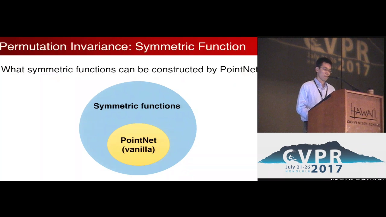
>> A very good question. Um it depends at which stage you are in the process essentially. Uh this is more linked with the second part. So the last chapter of this um boot camp which is touching on 3D machine learning and the goal is to have if you go in this direction you don't use algorithm per se. um well it's an algorithm but it's more you really need to make sure that the data that you provide on which the model is trained is of very good quality. So that means that if you take the process from scratch you will need to go through a labeling phase where yourself you will have to label at least the part of the data set and then use that to train your your model. So hopefully that answers your question, but essentially this is just a matter of um having a super nice data set and having a model that is able to pick up features from the data set to um to be distinguishable enough for different classes that you want to detect. These are some examples of what you can expect. Uh so this is with a segment OS solution, the region growing one. This is the unsupervised um like result that you you should get with plan based segmentation and then you can use each segment through a machine learning 3D machine learning model to be able to classify that if it's the ground if it's the um how do you call that the the pillon if it's the the the rebar if it's the the the the ceiling and things like this what can I show so this is an example of what you have um with open data Uh and this is also something with an automatic classifier right but that was trained on data with the various classes which is very interesting to get at scale or have uh color information that you can leverage. This is not always the case but this is what we show yesterday.
This is what you are able to recreate with what we had yesterday. This is not gion splatting right it's the point cloud but it's dense enough so that you can have a lot of information on on the various um aspects um this is another example maybe of unsupervised system right and what you see here this platform this is one of the thing I was talking about yesterday when I say creating assets and apps this is something that I initiated in 2014 for the lens surveyors in France. Um and that is still really relevant to uh make sure all the data is centralized but essentially the tech stack behind is not very far from what we are seeing today.
It's just the way of managing everything which is handled in a in an engineering way with modules and blocks that you can um have tied in together. This is one thing also um we'll speak about that a bit later. This is a self-supervised system where we use ontologies to know that cars are parked in the line. And this is fully automatic. So this is with Jeanjac that we we did that in 2020.
What else can I show? Um yeah, I think that's pretty much it as far as um as a point cloud and such goes.
Is there anything else that you wanted touch on before making a little u little pause maybe?
>> Yeah. Do you hear me? Yeah, I just wanted to know how how long and um how many time does it take to to get some uh train algorithm or how many files you need to uh with normal uh segmentation um just to to start working on on more messy file.
>> Yeah, great question. So if I take back uh this fully insupervised so you don't need to train anything. So it's just the time that we ingest is in conceiving the algorithm and fine-tuning the algorithm through the segment OS you have that and the implementation is there. So it's just a matter of understanding what you do and using it after but you don't get directly the classes and you need to work from there. Um so you have a labeling phase but you don't work at the point level you work at the segment level. Now the second stage is creating your model that can classify in various classes. Uh do I have one somewhere like here for example? It means that so not in this case but in normal case and what we will see just after we need to label a data set so you can use cloud compare or anything else the process that we did to try to be as quick as possible to generate uh data set. Usually it's a good rule of thumb to have a thousand object per class um for good quality detection. The trick is that if you work at the point level, you can you have a lot of point for one class so that you can diminish that. The other thing is uh you need to make sure that you have a balance between the classes. So here it's not bad because you have a lot of cars, you have a lot of trees, you have a lot of building and the ground but you don't have a lot of poles. So this is likely to be poorly detected. So essentially um to build a model you can expect like at least the first hand model and then you can refine iteratively. But you can expect if you have the data if the data is organized uh well you can expect to to spend between one week and a month on the labeling effort to constitute your your data set. This is not necessarily fun work. You have some tools that allows you to accelerate that but you have still to go onto the quality check because if it's not good quality you will not have a good model. Once that is done this is what we will see just aftera building the model uh is not very hard. Uh and this is a bit the novelty with this new datadriven approach is that the focus is not into the expert knowledge around the algorithm but the expert knowledge around the data to be able to make something really nice. and hopefully have an algorithm that you pick on the shelf more or less that will work good for your case. So this afternoon we will see several uh classical machine learning ones. You can expect to have very uh decent result with that at any point if I will speak about the threshold when to switch to a new algorithm or when to continue labeling this kind of things. This is really dependent on the score that you will have. But usually it's um good to have in mind that if after the first passes uh your data set is labeled, your model is established. If you have something that is above 80% in um global accuracy over all classes, then usually you are in a good standing to have something that you can push in production with the current model. If you are below that sometime we need to to investigate other models um deep learning ones to make sure that this is something that we can achieve. Hope this answers uh your question.
>> Yes. Yes. Perfect.
>> Okay. Awesome.
AF you wanted to to say something.
>> Um hello. Yes. U so I have just a question. So let's say for example we don't have labelled data for the 3D data but instead we do have label data in the 2D space.
>> Is there a way to go from the 2D to 3D?
Do you think like we can just segment 2D images and then do but I'm not sure if >> I lost a I lost a bit the end. I I I got the beginning.
>> Hi. Hi. Hi.
>> Yeah, I can hear you.
>> So I'm just asking about the if we do not have labelled data in the 3D space and >> instead you have the label data in 2D space. Should we segment the 2D and then do the reconstruct the reconstruction or is there kind of a trick to go between the two?
>> Yeah, you have tricks. Very very good question. So um do you have the link directly between the 3D and the 2D?
>> Uh what do you mean by link?
>> Do you have the position of the 2D image uh based on the 3D?
>> Yes.
>> Um yeah indeed it's just a matter of making sure that you have the position of your image based on your point cloud.
And what I really recommend then is essentially if you have the labels in the image space, you are in a projection um um let's say um setup where the challenge is having a projection that is uh as sharp as possible, right? So this is actually super cool stuff and this relates to um a field that I like which is called semantic photoggramometry where you actually uh label images and you classify your point cloud based on your images and the pose estimation. The only thing is the trick is in that case because you have a multiv- view setup you need to make sure to fuse prediction uh for a same pixel right you need to fuse prediction uh if you have not a setup with multiv- view so if it's a single view usually you will want to go into a autographic projection and have some kind of ray casting mechanism to check the depth so that you don't label point that are behind uh something if this makes sense you you've heard of the segment anything model.
>> Oh yes.
>> Yeah. Okay. So um this is something that I can also share. Uh so this is also part of some course but I have a tutorial there. It should be the tutorial section.
Uh let me share the the friend link to that because in it you have the projection equations that I already wrote. So um okay. So this is one example. You have an image. This is the result of some uh the only thing is which projection you use. That's what I'm saying. If you have only one image, just the autographic one is the one that you should use and you will project. So you have to use the masks uh maybe not directly the the pixel color values but masks underlying. So attach to each pixel your mask of the class and use that that you transform your point cloud. But this is essentially um some ways to do that and you have all in the okay so that's the spherical projection and the mapping the mapping I put it somewhere around so you get a here I do that with the color but you will have to do that with the masks um to get the the mapping and this is what is done for example that was the 3D point cloud put in a spherical projection on top we can use SAM here to to detect the various component and then The last stage is to back project that to the point level. So this is what is here. Um and you get that but you have to filter out the points that are not seen from a specific point of view. And if you want to label the entire scene, it means that you need to generate different point of views. The data sourcing that you know how to do preparing and featuring also and how to handle large data set. We have something. So now the idea is to try to build a predictive model with AI and that's what we are going to do just next. Beautiful. So now that we have completed this eight stages, the next logical step is to dive onto 3D machine learning. So this is something that I will also share in um this specific channel at any point. This is already ready and available for people at the academy. If you want to head straight on there, just please do so. I'm always super welcoming to new members there.
But if you are um happy to wait then maybe in the coming weeks, coming months, you will also see that happening. Have a fantastic day and see you in the next video.
Up Next

4:32
RANSAC: Random Sample Consensus in 5 Minutes
@CyrillStachniss
79K views•2020-04-25
87:26
Introduction to Secure Multiparty Computation with Yehuda Lindell
@fhe_org
7.7K views•2021-02-04

4:55
HTTP Requests Explained: GET, POST, PUT, DELETE
@codecademy
103.1K views•2021-10-07

19:25
Enigma Machine Mechanics: WWII Encryption Explained
@JaredOwen
13.2M views•2021-12-11
Related Study Plans & Knowledge Roadmaps
Structured learning paths in Computer Science
computer-science
Container Runtimes: Namespaces, Cgroups & Go
01Linux Systems & Go Programming Foundations
02The Core of Isolation: Chroot and Filesystems
03Linux Namespaces: Process Isolation
+ 3 more learning modules
32h6 modules
Explore Roadmap
computer-science
Building a CHIP-8 Emulator: Rust & CPU Basics
01Computer Architecture Foundations (Bits & Bytes)
02Rust Programming for Systems Development
03CHIP-8 Virtual Hardware Specifications
+ 2 more learning modules
32h5 modules
Explore Roadmap
computer-science
Building BitTorrent: Go, P2P & Concurrency
01Go Fundamentals & Concurrency
02Networking Foundations & P2P Architecture
03Bencode Parsing & Torrent Metadata
+ 3 more learning modules
26h6 modules
Explore Roadmap
computer-science
Actor Models (C++ Concurrency & Lock-Free)
01C++ Multi-Threading Foundations
02Thread Pools and Task Scheduling
03Atomics and Lock-Free Queue Design
+ 3 more learning modules
45h6 modules
Explore Roadmap