


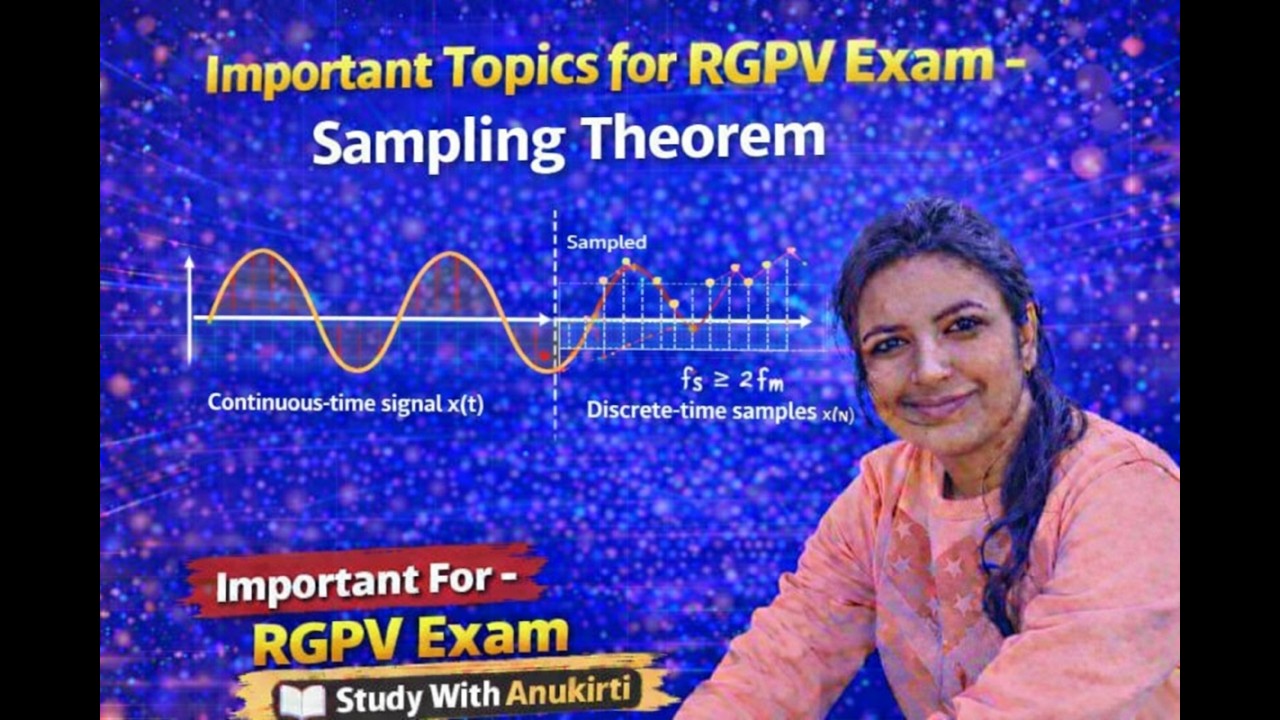





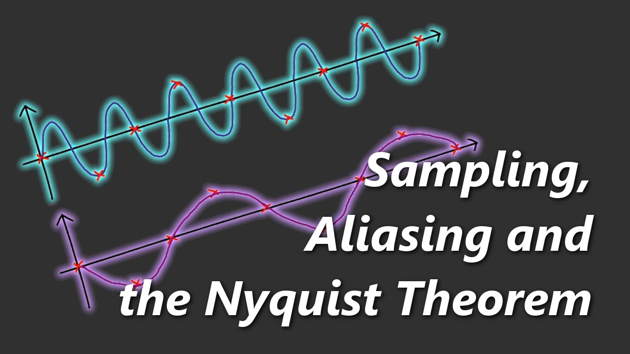




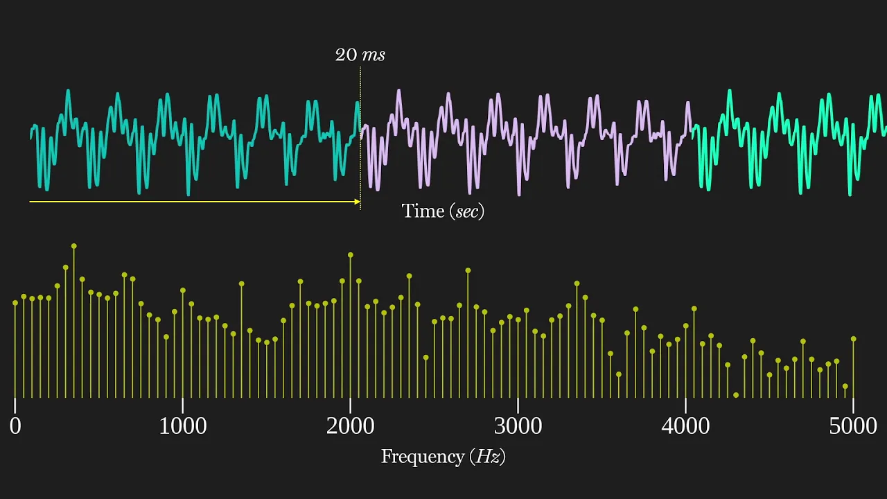



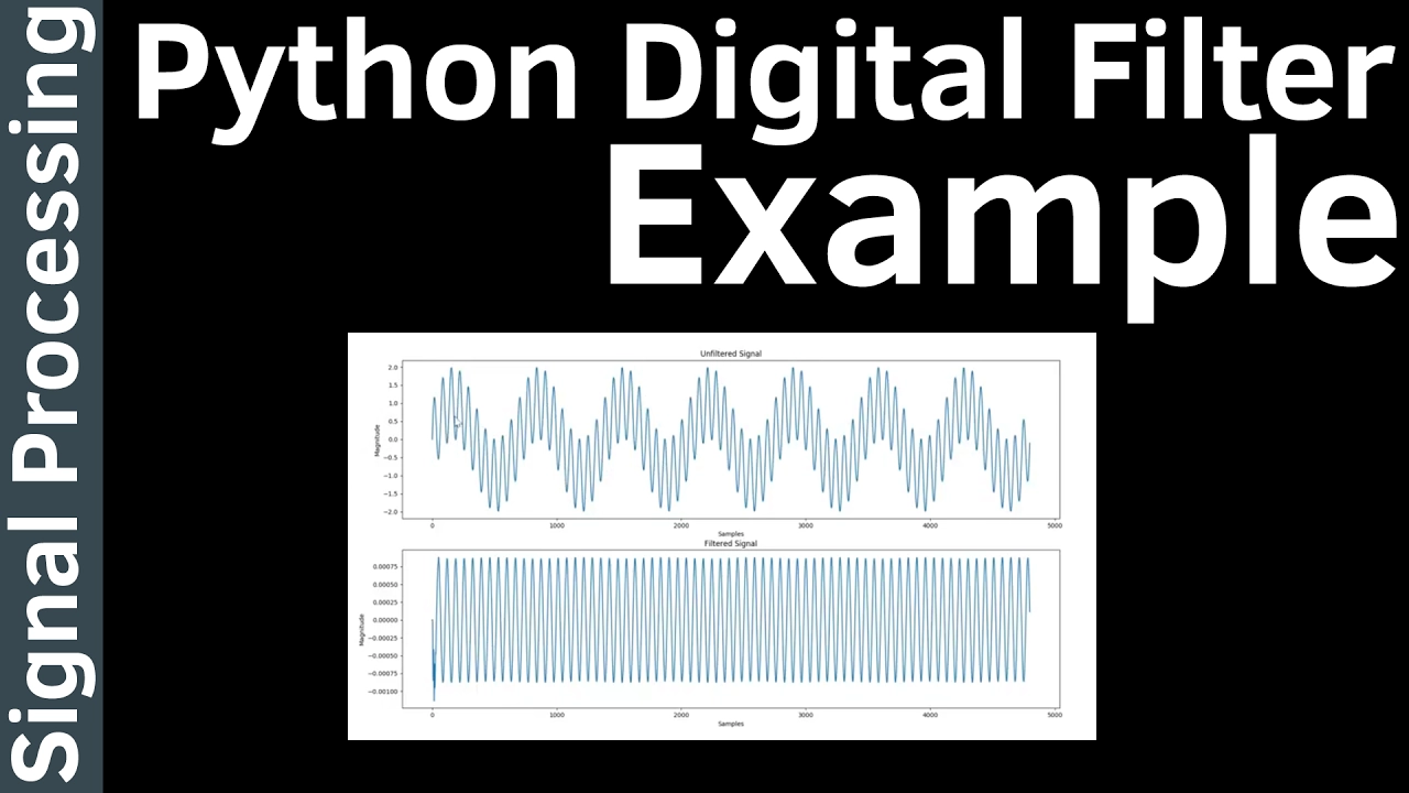




This video demonstrates how to compute the Fast Fourier Transform (FFT) of a time-domain signal using Python's numpy.fft.fft function and plot the resulting frequency spectrum using matplotlib. The process involves three main steps: (1) constructing a time-domain signal with specified sampling frequency, signal frequency, and number of samples; (2) performing FFT to obtain complex frequency coefficients, then calculating the magnitude and normalizing by dividing by the number of samples; (3) plotting both the time-domain signal and frequency spectrum, with the latter requiring application of the Nyquist sampling theorem to limit the frequency axis to 0 to half the sampling frequency and proper handling of the DC component. The video shows examples of single-frequency and multi-frequency signals, demonstrating how FFT reveals distinct peaks at each frequency component with magnitudes proportional to their amplitudes.
Computing FFT and Plotting Frequency Spectrum in Python with NumPy and Matplotlib
Added:hello everyone today's video i have two goals the first goal is to demonstrate how to compute a fast fourier transform using the numpy fft function in python so i kind of assume that you know what is a fast fourier transform so today i'm focusing on how to calculate in python using numpy module second goal is to plot the frequency spectrum of the output of the fft using map.lip so i hope you find this video helpful so we do it in three steps so first we will construct a time domain signal so this is the the input signal we are going to compute the fourier transform so normally it can be a sound signal or any kind of time dom a sensor signal any kind of time domain signal right so second step we will perform fft right so lastly we will plot the both the time domain signal and the frequency spectrum first thing we do we're trying to construct a time domain signal let's say we have a sampling system so we have sampling frequency of 2000 kilohertz so this is the sampling frequency so we're going to build a time domain signal so so this t step this t step uh is the sample time interval we need this input signal frequency let's say for the moment we assume that i have a sine wave signal an ideal sine wave signal with a 100 hertz frequency so this is my uh signal frequency okay so then we will so this this is the number of samples of the signals okay so then we need to construct a list for times timestamps so we use the numpy linear space function to create so it will be from time 0 to t step okay so we have n data points oh i've forgotten to import the input module so first thing you do is you need to import numpy as np later you also need a map lib to plot so so this is the time steps are timestamps of the time domain signal so we compute fft there is a frequency interval for each frequency bin so if you know the theory it's basically uh the trampling frequency divided by the number of samples right so if you don't know why i recommend you to do online research so this is a frequency interval similarly we need to because we need to plot the uh frequency spectrum so we need to create a x-axis for the frequency spectrum which is a list of frequencies so again we use the numpy linear space function to create this so we can do similar things like the timestamps except that we change this to the frequency intervals okay this is the frequency steps okay so lastly we just need to uh create a signal so we're going to create a sine wave signal so i'll call it y is our signal input time domain signal so i have an amplitude of one a sine function so i need a frequency of frequency of 100 hertz right so i will just compute that 2 times pi 2 times pi times the frequency and the time steps so this will be our signal so basically what i've done is i created a time series with the interval of t steps and then i created a sine wave using the numpy sine wave function so let me plot that for you to quickly show so here i plot one cycle of the time domain signal so let's do this plots okay for the moment we just have a one row and one column for the plot okay so we simply plot the time versus the signal okay you convert this into an integer okay so let's run i forgot to show show the plot here so now you can see uh i've created a time domain signal so x axis is the time y axis is a signal signal so probably clear so now you can see those are the discrete time data points here those dots okay wait a moment okay so next we will perform the fft uh using the numpy fft function so it's actually quite easy so it's simply using a numpy fft fft so you just simply pass in the input time domain signal here so the details about this function you can refer to this website for the numpy fft function let's go back so this will give you so x will be a series of uh complex numbers so this isn't the definition of the fft so you get a complex number as the output so for now we're only interested in the magnitude of the of the fft output so you just do an empire you just take the absolute value of that also you need to normalize the the magnitude right you need to normalize magnitude by the number of samples here so in this case it's basically n okay so now technically we can plot we can plot the frequency domain also so here i just need to add i we need to add uh more one one more plot so let's say let's do it this way so i'm gonna have two rows so okay so here we plot the frequency the uh fft output which is fft magnitude versus frequency so now you can plot so you see now you basically what you're seeing is the frequency domain in the in the second plot here so the x-axis is the three is the frequency and y-axis is the magnitude but it's not that correct yet so in fact you can see that if you know about the sampling theorem so so if you have a sampling frequency of 1000 2000 hertz so you're able to reconstruct your signal below half of this frequency which is one 1000 hertz it's called the nikoi nyquist sampling theorem so what we'll do here we will do more small modifications so we are only going to plot half of the frequency of the sampling frequency so we will create another x-axis for the frequency so it's going to be from zero to half half of that okay into plus so i already know that you need to convert it into integer because there is a python list index and you need to plot the okay with x magnitude for the plotting so it's basically two times the original one so max max so one point one node need is a dc component we don't need to multiply by two so we just need to divide divided by two so i am not going to explain why because i'm not really good at that so but just to say you need to do this otherwise you end up having a wrong dc magnitude as you will see later dc component 2 okay so now we can plot the proper plot proper frequency domain signal so now you can see i'm only plotting up to 0 to 100 1000 hertz and my signal frequency is actually at 100 hertz so the magnitude is 1 which is exactly what you see here so my signal frequency is 100 hertz and the magnitude is one we get more uh fine resolution in the frequency domain you just need to increase the number of samples let's say i have 10 cycles of samples now you can see this is my time domain signal and this is the frequency spectrum so you can see at 100 hertz here i have a magnitude let's say i have uh my signal has two frequencies for example i have a another frequency which is let's say three times the three times the input frequency original infrequency let's say 300 hertz so i multiply 3 here so it's probably easier to understand if i put it here and i have magnitude of a of a 4 for example so if i run this so you can see that this is my time domain signal it has two frequencies and it is clearly shown that on the frequency domain at 100 hertz you have a component of a magnitude of 1 and at 300 hertz here you have a magnitude over 4. so again we can add a dc component let's say i have a dc signal over 2 so i run it again now you can see the dc which is a zero frequency here has a magnitude of two remember just now i have divided two back in in the previous calculation here because in dc you don't need to multiply by two here so i divide the two back here so lastly let's try to make the plot uh more beautiful so we'll first we will put some labels on the axis so set label x label so the first is will be the time so the unit is the second and the label for the second for the frequency spectrum will be a frequency so it will be in hertz and okay you can turn on the grids also all right see you again so now you can see this uh you see you see this uh x label here and i turn on the grid okay so let's try to set the limit of the axis also just to make it even better so let's say just to limit that try again oh what's happening okay so this should be x two here yeah now you can see i've limit the the x x axis so it looks a bit better so i'm going to remove this second frequency here so i can have a single frequency all right so you have a single frequency look look at that okay you can see the label here cannot be seen so let's make a change so i believe we can try this uh tight layout function here here we go so now this is of this the final result so basically we have uh created create a time con time domain signal which is here and we have compute fft then plot the frequency spectrum here so i think it looks quite good i hope this video is helpful to you thank you for your time bye
Up Next
Homography in Computer Vision: SVD & RANSAC Explained
@Foo-i1v
74.9K views•2018-01-07

Homogeneous Coordinates in Robotics | Cyrill Stachniss Lecture
@CyrillStachniss
80.8K views•2013-10-22

HTTP Requests Explained: GET, POST, PUT, DELETE
@codecademy
103.1K views•2021-10-07

Enigma Machine Mechanics: WWII Encryption Explained
@JaredOwen
13.2M views•2021-12-11
Related Study Plans & Knowledge Roadmaps
Structured learning paths in Computer Science