
















Homogeneous coordinates are a mathematical representation in projective geometry that allows expressing geometric transformations (rotations, translations, scaling, shearing) as single matrix multiplications, enabling efficient chaining of transformations in robotics and computer vision applications. A point in homogeneous coordinates is represented as a vector [x, y, z, w], where the Cartesian coordinates are obtained by dividing by the last component (x/w, y/w, z/w). Points at infinity are represented by setting the last coordinate to zero. This representation simplifies coordinate frame transformations and is essential for handling camera projections and robot kinematics.
Homogeneous Coordinates in Robotics | Cyrill Stachniss Lecture
Added:Foundational Linear Algebra, specifically matrix-vector multiplication, matrix inversion, and the identity matrix.
Basic 2D and 3D Cartesian coordinate systems and vector representation of points in space.
Elementary trigonometry and the representation of 2D rotations using rotation matrices.
The conceptual difference between rigid body motion (translation and rotation) and non-rigid transformations.
Forward and Inverse Kinematics for robotic manipulators, including Denavit-Hartenberg (D-H) parameters.
The Pin-hole Camera Model and projective geometry used in computer vision and camera calibration.
State estimation and pose tracking in SLAM (Simultaneous Localization and Mapping) algorithms.
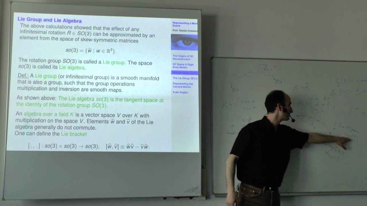
Introduction to Lie Groups and Lie Algebras, specifically SO(3) and SE(3), for advanced 3D rotation and rigid-body motion representation.
80.8K views657likes28:34Original Release: 2013-10-22
okay so then welcome to the course today um today as announced yesterday will only be a quite short lecture um on homogeneous coordinates which is one way one alternative way uh to using the um uking coordinate frame which is frequently used in robotics to express Transformations and that's something which the students of last year said it would be nice to get an introduction on that and therefore we have a short whatever 20 to minute probably introduction to homogeneous coordinates and what they are used for what we can do with that why they are kind of a useful tool for us and you will Theos homogeneous coordinates especially Transformations expressed in homogeneous coordinates um throughout the lecture a few times so that you know what you're going to see after that we will have in one hour exercise um kind of an introd short introduction to matlb or octave which we will use in the course and then directly exercises with this homogeneous coordinate that you see here so after half an hour lecture approximately 1 hour of tutorial and then from next week on we continue as planned every Monday is a lecture and um Tuesdays from 10: to 12 is the tutorial okay so let's start why are we why I why do I claim that it makes sense to leave the cartisian world um the reason for that is that a lot of Beering only sensors that mean sensors which do not measure the distance to obstacles but just the um the orientation where an object is such for example a camera camera doesn't give you any distance information by counting the pixels or by knowing which pixel corresponds to which angle you can estimate at which angular orientation an object that you perceive is located but from a single image you can at least if you don't integrate any background knowledge or any additional information cannot tell how far a point is away and that means that the camera generates a projection of the 3D World onto a 2D image plane so just it's a projection of any 3D Point object whatever it is onto a 2D image and um the ukan geometry is actually suboptimal to describe that we can do that so it works it's nothing which kind of hinders us from doing that but it's suboptimal in the sense that the mass can get a bit complicated so the equations for doing that are suboptimal especially for describing the central projection that is you have this is probably the camera model you've learned at school so you have one center of the projection and every point that is projected On a par on an image plane which is parallel to the um Optical axis go through that uh point and um as I said the ukian geometry if you express all that in with ukian math it can get a bit complicated and therefore people introduced another space that this or another kind of geometry which is called projective geometry which which explicitly handles this or is kind of well suited to handle these projections and as a result of that the mass becomes easier and therefore it makes sense to actually look into that representation um it should be noted that the projective geometry doesn't change the relation between objects and space so we can repres we we model the same relation of object in that space um the only thing is that um as I said that the math becomes easier Transformations especially that's what we are interested in can be handled easier um in kind of a very nice and simple form and that's kind of the reason why we use that and we look especially into homogeneous coordinates and homogeneous coordinates is a coordinate system um used in projective geometry and um it has two nice advantages the first one is that we can represent what we call points at Infinity in a very nice way points at Infinity are points which are infinitively far away but where know the distance if you think of a camera You observe an object um and you know which to which Pixel It corresponds the object you know the angular orientation of that object relative to to you but you have no idea how far it is away and um it can be that this point is infinitively far away if you think about your general representation of space with X and Y coordinates it's actually not easy to describe a point which is infinitively far away or points at Infinity especially you cannot do that um with um an finite coordinate so you can whatever compute have an additional factor which goes to infinity and then you take into account the angular component and then generated Point Infinity but that's kind of not that nice um in contrast to that the homogeneous coordinates explicitly allow us to represent points at Infinity the second thing that's the thing which is kind of most important for us in this course here um is that we can use a single Matrix to represent a Transformations so it means um Transformations which include rotations translations um sheer um scale changes we all can put that into a single matrix multiplication and that's what makes it very very easy for us to do that if you think about the 2D geometry and you have the vector in 2D you want to transform this Vector you could do that for rotation so you could take a rotation Matrix multiply it with the vector and then you got the rotated Vector but couldn't do that with Transformations and so in the homogeneous coordinates the whole uh Transformations we can actually or not the whole Transformations but um the um projective transformation which include also the a Transformations which include also translation rotations can be nicely put into a single Matrix and that means by single simple Matrix multiplications we can express coordinate Transformations which is really nice and that's actually the main reason why we do that so although points Infinity are very important um this is nothing which will be densely covered in this course uh but the last Point here that's something which we will use frequently in this course um and therefore it makes sense to know what homogeneous coordinates are okay let's go a bit more concrete what is a homogeneous coordinate the represent representation of X of an geometric object it's just a point for now is homogeneous if x and a scalar Factor Lambda mply with X represent the same object given that Lambda is is not zero so we have some Vector x and x as well as any scalar multiplied with X should be exactly the same object so that's just the definition one example for that is we have a point x which has three coordinates U V W If U Can be expressed as W * a new variable X V can be expressed as W Times a new variable y then this point and this point xy1 represent exactly the same object because you obtain this one over here by multiplying this term over here by 1 / W so UV W is equal to xy1 * 1 / W and this is exactly the Scala Factor okay okay so what can we do with that so this is our homogeneous Vector exactly the same equation we had before and in and this should correspond to the point XY in the ukian space so if I want to go from the ukan space to the homogeneous space it's sufficient to add another dimension to my vector and add a one down here the new dimension I add so for representing objects in the 2D World which I used so far a two-dimensional Vector for I need now a three dimensional vector and to map from the ukan space to this homogeneous coordinates I just add a new dimension and this Dimension takes a value one that's all I do okay and then I can if I I have a point in homogeneous coordinates U V W over here if I want to transform that one to the cartisian space I just take the last component and divide all elements by the last component just kind of normalize it um by dividing the whole Vector through one one divid by W therefore this value gets one and then I can neglect this component one and this gives me my point in the ukian space okay so we can visualize this now if this plane over here is our is R2 so our regular CES in two- dimensional space and the three-dimensional construct here is um represents my um homogeneous coordinate system then this R2 is just a plane at the last coordinate so the Z coordinate equals one so that's one in that threedimensional space and our point x in um the edian space say our Point XY down here is exactly this point this single point in the plane in my threedimensional space this represents any object that lies on this on this line which go through the uh origin of the coordinate frame through that point x further on and this is exactly this um this Lambda this scaling factor that I add so if my point x lies in my homogeneous space over here that means it is exactly the same unchanged Point um down here in my uh so kind of in R2 in my two dimensional cartisian space and you may see that that wherever this point lies on that line it will fall exactly on this coordinate in a 2d plane and this is why maybe you may be able to see the connection to for example a camera wear point which somewhere lies on line gets projected on one specific point in my image plane so if you want to map from any point on that line we just divide all coordinates by the third coordinate that means the third coordinate gets it's one so it moves down here on that plane and then we have our coordinate in the um cartisian space so from with normalizing we go to the cartisian space if you want to go from the Cartesian space to the um homogeneous space we just have to add a new dimension and put a one in there is there any question about that okay at the result the center of the cord frames are 0 0 and a one another component so whatever value I put in there I put a two in there would represent the same object if I normalize it through um the first coordinates because they are zero so 0 01 or 0 z01 are the centers of the coordinate frame and this allows us now to express points at Infinity so points which are infinitively far away this Cas is quite easy by just taking our coordinate U and V and add a zero down here because if you want to map this now to the ukian space we would need to divide u and v by zero and if you let's say take a value which we let approach there mean this point moves away on that infinitively far away on that line and so by explicitly having a zero in here we can represent points that are infinitively far away and um the the nice thing is that we can do that with three coordinates here which are finite so we don't need infinite large values down here as we would need to do that in the um in the cartisian world we can now do certain things like checking if we can express lines in a very similar way and can then easily check if lines are parallel or orthogonal um without caring what the individual Dimensions actually look like and that's kind of a very nice property that's what it's often used for if you work as cameras and want to take into account points which are infinitively far away there's nothing we do here in that course at least to not to a great extent and therefore um I don't want to go more into the details here um I just want to look more on um the Transformations that we can you express with those homogeneous coordinates because that's something we are going to use here in that course okay so the first thing we can do um we can also do that for 3D points we just have a than a four-dimensional vector which is here the additional value T then we normalize by T so we have u v w t and exactly the mapping to thean space and again if we M map back we have our values here we just add one down here and we are in our homogeneous world so the maping between Both Worlds actually quite easy okay so how can we describe Transformations using this um coordinate system um I said you before that we can express everything Thing by a matrix transformation uh the only thing is this Matrix should be invertible so we have if we have our transformation matrix M and we multiply an ector x with m in homogeneous coordinates we get another Vector in homogeneous coordinates X Prime over here and what I want to illustrate now that we can actually by having a special structure in this Matrix M we can express a lot of interesting Transformations um that we cannot express with the single Matrix of operation in the regular cartisian space so we need to have a more complex transformation and here we can nicely put that into one single Matrix then Express this with a single Matrix so how does this Matrix look like so assume we have the we are living in the 3D cartisian World so we have a 4D vector and therefore a 4x4 Matrix over here there our Matrix M so this should indicate that it is a 4x4 Matrix and the first thing we want to do is we want to express trans transtions um so just pure translations in this space that was something we couldn't do in the ukian space by a matrix transformation we would have to add a vector to a vector but we can't um in the in the cartisian world we cannot express this by a matrix multiplication this is how the Matrix look like so our Matrix M has any scale of scale factor this doesn't matter because we're living in the hom in the homogeneous coordinates so the scale foror can be any value and then uh M has has this form this guy over here this I is an identity Matrix and especially a 3X3 identity Matrix so it looks like this this value here is simply a vector of zeros threedimensional Vector of zeros transposed so that's kind of um here three 1 2 three zero values that's regular one and this Vector T is a translation Vector this translation Vector is has three components and the translation X the translation in y and the translation in that so it exactly looks like this and we if we build up our Matrix in this in this way we can multiply our transformation matrix M with any Vector we will get a new Vector it has exactly the same values but it is translated the X component by TX the Y component by Ty and the V component by TX okay and the N thing is we can do this with a matrix operation we don't have to add a vector as it would need to do that in the cartisian world so there's nothing bad about adding a vector just to say that but the ni thing where we can express everything here with one Matrix operation so if you combine that now with different forms of transformation like rotation matrices or different things um then it's inconvenient if you always have to have a multiplication and then add something and then if you stack them or chain them all together these uh Expressions can get a bit ugly and um here everything is done in Matrix form I can just multiply my matrices um and then in this way um execute for example a large chain of Transformations okay so trans translation is nice but typically we also need to rotate things in space so what happens if we want to express rotation um as well want to express a rotation so if you want to express a rotation our Matrix M looks like this again we have our zero down here we have our one here this now is again uh a zero Vector with three elements so this was the vector where the translation Vector was sitting before so this is zero that means we don't have any translation in here and here we have a matrix R this R is the 3X3 Matrix this is a regular transformation uh rotation Matrix as you all should know it from the um cartisian world so rotating about around an axis X Y in case you forgot how this one Matrix looks like I have one slide to remind you on how these matrices look like so in the 2D world it's easy we just have one axis of rotation around we can rotate and so if you want to rotate a vector X um around uh the center of our coordinate system with uh let's say one angle Theta here we can express this by this rotation Matrix multiplied by my Vector X and the output I get from that is this rotated Vector X so even in the CES world we could use a standard rotation Matrix to express rotations of um of vectors or of points in the 2D world this is familiar to everyone is familiar with this concept right everyone should have heard that perfect okay this was for the 2D case in 3D it gets a little bit more complicated because we have three rotation axes you can rotate on the xaxis yaxis or that axis and there are a large number of different ways on expressing transformations Sol around which which AIS should I um translate or rotate first or how how where are the AIS or do I only have one AIS um which can lie have any arbitrary uh orientation in space so different ways for expressing uh rotation in 3D there's just one way for doing this these are the standard transformation matrices so this Matrix over here expresses a rotation in 3D around the x-axis with the angle Omega so this one stays constant so here's a one in the in the X in the First Dimension which represents X because I rotate around the xaxis so a point on the xaxis is not changed and I have exactly the same rotation Matrix I had in here um in the two other components and we in a very similar way we can do that for y and for the Zed coordinate um here that coordinate is one and here you have one in the second dimension and this gives you three different rotations one around the x-axis one around the y axis one around the Z axis and if I want to express any rotation in 3D I can actually do that by with three rotation matrices so rotation about x y and that just multiplying them here you can already see we have three rotations we just multiply these matrices we get a new Matrix which expresses the rotation around all three X's that's something which worked in the Cartesian world but only for rotations not for translations and in homogeneous coordinates we can now use this also taking into account um the translations okay so going back we have for our simple rotation as we had before we have our rotation Matrix R which is exactly this R Matrix over here or this Matrix over here depending if we in 2D or in 3D and that's the way I can express a rotation and now we can actually combine both we can take into account a translation and a rotation and this Matrix looks like this so we have our Matrix R here this was where the identity was before when we look about translations the translation Vector here and the the the bottom row is not changed this is now has now six parameters so we have three parameters in the rotation three par parameters in the translation and that's kind of a rigid body transformation or a motion transformation over there called and that is the thing we will use frequently in this course so to for example we have a measurement in the coordinate frame of the robot of the sensor we may need to compute where this point now given that the sensor is not mounted exactly at the center of the robot and given that the robot is somewhere in space so we can actually Express this by multiple coordinate Transformations so first um from the in the from the sensor frame to the center of the sensor then from the sensor to the center of the robot and then from the center of the robot to um the point in the world depending how one expresses we have to do that a forward step or a backward step so um that depends on what we actually want to compute um we can however do more so at least you should know what else you can do with that so we can have soal similarity Transformations which have another dimension and this Dimension scales the object so we can make an object smaller or bigger and this adds a scaling Factor M here in front of the transformation matrix so it's not we cannot multiply it here in front because that would be normalized away because then M would one would be also not multiplied with M then this is not the case since we don't want that we have to put our M here so if we do it in that way we can um actually have um so we can actually scale an object and we can also have a Transformations which have 12 parameters then we just have a matrix a over here um which has nine parameters and these nine parameters um also include different scale parameters and also Shear so you can Shear objects there's nothing we're going to use here but we can actually use this we can use this um the tool of homogeneous coordinates this coordinate frame to express this in in very elegant way just by a by a simple Matrix then we can just multiply multiple of those matrices with each other this way we can chain those Transformations and then take the resulting Matrix multiply a vector with this Matrix and then obtain the final transformation just as an small overview in the 2D world because it's easier to visualize you have all the different types of Transformations so you have a simple translation this is again here we have the identity Matrix in this now 2 by 2x two block over here and our translation X and Y um we can actually mirror object at the uh at the y- axis then this guy gets negative we could do the same with the x-axis if you would like to um we can have a rotation so we have we have our rotation Matrix over here again this is R um we have can combine the rotation and the translation so with the rotation Matrix over here and the translation Vector over here in the 2D worlds again that's something we are going to use here and then you have multiple things like scaling the objects additionally and um you can even have a scale difference in the different X's if you have a different scale in X and different scale in y you can Shear symmetric Shear that both exes are sheared in the same way or an asymmetric Shear this is not the case a fre Transformations or general um projections so we can put do all of that in this nice space so if we have our Matrix M here which we can do a transformation the next nice thing is um is that we can actually invert our Matrix to get the inverse transformation so if I carry out a transformation by multiplying m in X I want to kind of want to undo that operation I can multiply the resulting Vector so with m m to the^ of minus one X Prime gives me my original Vector X that's really nice because this way I can actually also invert transformation very very nicely without needing to go into the details of the transformation we just need to invert The Matrix yes please and this our M always invertible m is always invertible yeah so this this results from the way you construct those matrices that you have this one over here the zero Vector here translation goes here and this is a rotation Matrix the rotation Matrix is always invertible and as a result of that um you can show that this if you construct m in this way it is always invertible um yeah the only thing you need to take care of is that Matrix um Computing the matrix product is not commutative so it's something else if you multiply Matrix M1 with M2 or M2 with M1 so in general these two operations will not give you the same point because of course if you rotate first around the x-axis and then around the y axis you get a different result if you first rotate around the y- axis and then around the x-axis so the order in which you conduct these mrix multiplications needs to be taken into account this is just different transformation that you appli something else if you or first you have this object here and I can either rotate it first and then move it somewhere in space or I can move it somewhere and then rotate it depending on as I three rotations different results may be the output okay so said about that and again just to wrap that up the the thing which you most use in this course here is um expression of motions so we have a rotation Matrix with three components and a translation Vector with three components so we have six components we express the motion of objects in um the 3D World or if we only in 2D there just one rotation and two translations exactly the same form except that this would turn into a 2 X2 Matrix and that's what we're going to use extensively in this course there's no kind of black magic behind that and I hope you in the next hour will Ex explore that a bit more on your own computers uh with octav and fabito will take care of the exercise and guiding you through that process so that you get used to this concept and um and feel comfortable with that so to conclude um homogeneous coordinates adjust an alternative representation to the edian space uh for geometric objects and it is a coordinate system which is used in projective geometry the important thing is that I have um objects or geometric objects vectors and they represent the same two vectors represent the same object if they just uh if they are just scaled so if I have X is equivalent to any Scala time x as long as the scalar is not equal to zero that's kind of the the important definition in here and um through the extra Dimension that I have um a lot of Ni things can be represented like points and infinity through this extra Dimension I can also integrate rotation translation and all the other things you have seen here into Matrix operations um and in this way I can easily chain those um Transformations and that's the reason why we often use that um if you want to know more there are a lot of geometry textbooks or projective geometry which explained that actually found the Wikipedia page quite good as as a good introduction to read through that there are another references to longer tutorials um so if you just want to reread what I've presented here um there probably the EAS I put it here because it's for you probably the easiest resource to look up although there may be better descriptions but um I actually found it quite nice that's it from my side for today um are there any questions about that what you have seen here okay so that's it I hope a lot of questions will come up in the next hour when we do hear the exercise um yeah then we see each other next week on Monday thank you very much
Up Next
18:59
Homography in Computer Vision: SVD & RANSAC Explained
@Foo-i1v
74.9K views•2018-01-07

14:51
Computing FFT and Plotting Frequency Spectrum in Python with NumPy and Matplotlib
@1mviews876
120.4K views•2020-11-08

4:32
RANSAC: Random Sample Consensus in 5 Minutes
@CyrillStachniss
79K views•2020-04-25
19:25
Enigma Machine Mechanics: WWII Encryption Explained
@JaredOwen
13.2M views•2021-12-11
Related Study Plans & Knowledge Roadmaps
Structured learning paths in Computer Science
computer-science
Building a Rust Debugger: ptrace, ELF & DWARF
01Systems Programming Foundations & Rust
02Process Control and the Linux Ptrace API
03ELF Layout: Inside Linux Executables
+ 3 more learning modules
38h6 modules
Explore Roadmap
computer-science
Container Runtimes: Namespaces, Cgroups & Go
01Linux Systems & Go Programming Foundations
02The Core of Isolation: Chroot and Filesystems
03Linux Namespaces: Process Isolation
+ 3 more learning modules
32h6 modules
Explore Roadmap
computer-science
Building a CHIP-8 Emulator: Rust & CPU Basics
01Computer Architecture Foundations (Bits & Bytes)
02Rust Programming for Systems Development
03CHIP-8 Virtual Hardware Specifications
+ 2 more learning modules
32h5 modules
Explore Roadmap
computer-science
Building BitTorrent: Go, P2P & Concurrency
01Go Fundamentals & Concurrency
02Networking Foundations & P2P Architecture
03Bencode Parsing & Torrent Metadata
+ 3 more learning modules
26h6 modules
Explore Roadmap