

![線形代数[ゆっくり解説/数学]#01](https://i.ytimg.com/vi_webp/SJq0pZqlf_s/maxresdefault.webp)

















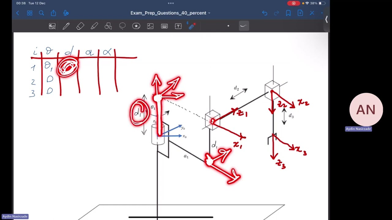








Robot kinematics involves calculating the relationship between joint angles and end-effector position/orientation; forward kinematics determines Cartesian coordinates from joint angles using homogeneous transformation matrices derived from Denavit-Hartenberg parameters (theta, alpha, d, a), while inverse kinematics solves for joint angles from desired Cartesian positions by first finding the spherical wrist center position geometrically and then solving for wrist orientation, with singularities requiring configuration values to resolve ambiguous solutions.
6 Axis Robot Arm Kinematics Tutorial: DH Parameters with AR4-MK2
Added:Linear Algebra and Matrix Operations: A solid understanding of coordinate transformations, 3D rotation matrices, and 4x4 homogeneous transformation matrices.
Basic Robotic Terminology: Familiarity with core concepts such as Degrees of Freedom (DoF), joints (revolute vs. prismatic), links, and end-effectors.
Trigonometry and Spatial Geometry: Proficiency in solving geometric equations and visualizing mechanical structures in three-dimensional space.
Introduction to Kinematics: Conceptual understanding of the difference between forward kinematics (finding position from joint angles) and inverse kinematics (finding joint angles from position).
Jacobian Matrices and Singularity Analysis: Learning how to calculate velocity kinematics, map joint velocities to Cartesian velocities, and identify kinematic singularities.
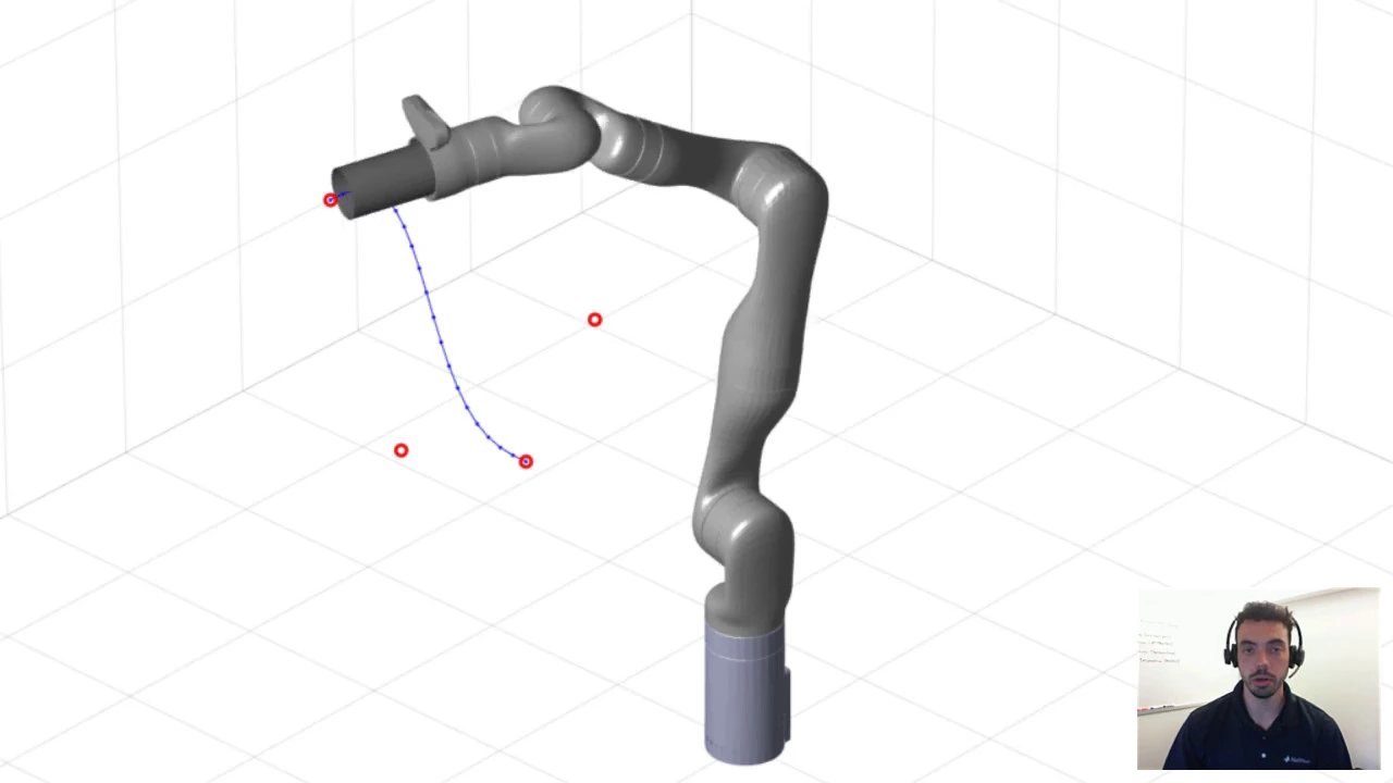
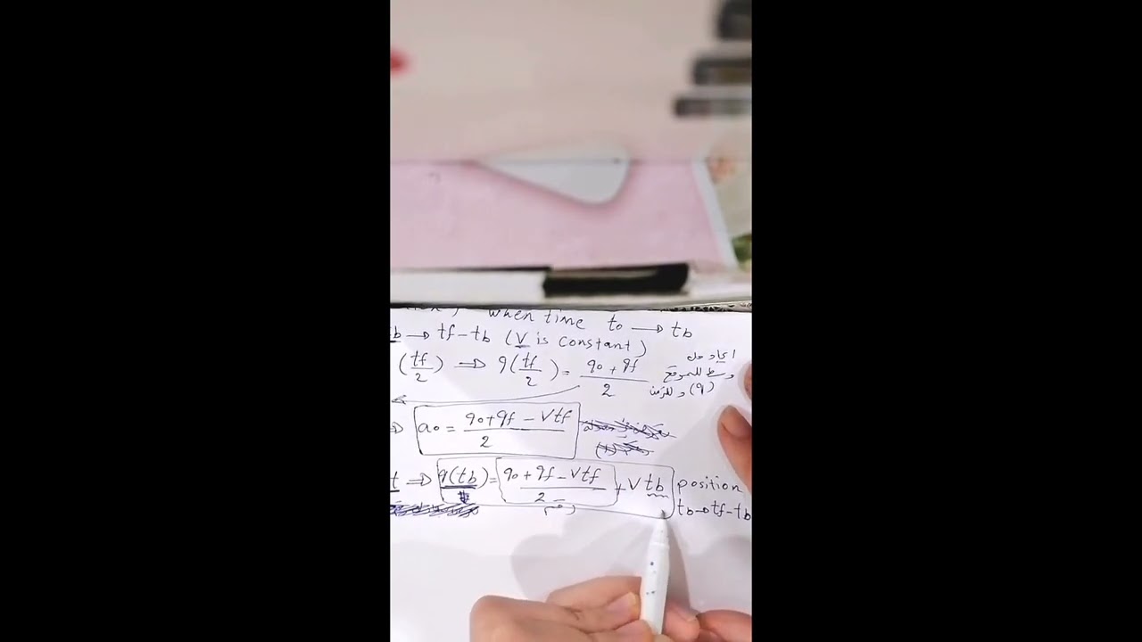
Trajectory Planning and Path Generation: Developing algorithms to guide the robot's end-effector smoothly through 3D space using cubic splines, Cartesian paths, and joint-space interpolation.
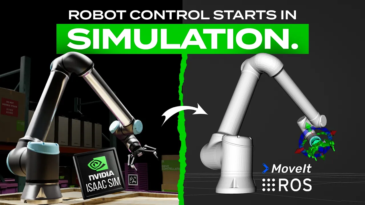
ROS and MoveIt Integration: Implementing the kinematic model of the AR4-MK2 within the Robot Operating System (ROS) environment to utilize motion planning libraries like MoveIt.
Robot Dynamics and Control: Studying the forces and torques (using Newton-Euler or Lagrangian formulations) required to actuate the joints, transitioning from geometric motion to physical motor control.
59.9K views2Klikes1:41:55Original Release: 2024-02-10
hey everyone I get a lot of questions on robot kinematics and how that works um so I wanted to make a new video to go over that topic if you've ever wondered how a robot arm with six separate Motors can all work together to make the ector go perfectly up and down in the Z direction or side to side in the X direction or rotate around a single point in space um that's what the robot kinematics do it's a lot of math involved in that and that's what I'm going to go over here if you've ever tried to study Sixaxis robot kinematics before or done a Google search on it you usually end up looking at something like this that has some diagrams some tables gets into formulas and before you know it you're looking at transformation matrices and you just end up more confused than when you started these are all usually written from the perspective of somebody who already understands it so I want to try and make a video that explains it you know for the rest of us that uh goes to a beginner level so I'm a visual learner I need to see the math I need to see the problem worked out in front of me so what I've done is I've uh put together this Excel spreadsheet where I have all the robot kinematics all worked out in front of me and I can change the values and see everything change and see how the formulas all work their way through um you can get this uh spreadsheet here on the ar4 project website here at Anon robotics.com if you come to downloads and then come down here to documents um we have the kinematic calculation sheet on this sheet on the left side I've got the forward kinematics worked out and on the right side I've got the inverse kinematics worked out so before we get into any of that we need to uh understand what is forward kinematics and what is inverse kinematics so to illustrate the difference between forward and inverse kinematics I have the ar4 control software open here and then I have a camera set up on the robot so you can see it move the forward kinematics are when I know what the joint angles are but I don't know what the cartisian coordinates are for the XYZ Off Pitch and roll position of where the end Defector is out in space so as you can see here when I jog the robot uh using joint mode changing the joint angles the forward kinematics calculates out and tells me what the XYZ yaw pitch and roll position of the robot is you can see every time I jog it the uh cartisian coordinates up update there now the inverse kinematics is the opposite that is when I know what the cartisian coordinates are but I don't know what the joint angles need to be to make that happen so when I jog in the Z direction for example if we jog straight up the inverse kinematic calculation is what figures out what the joint angles need to be to make that move happen so every time I jog in cartisian you can see the joint angles updating so that is the inverse kinematic calculation that makes that happen so now that we know the difference between Ford and inverse kinematics I'm back on the spreadsheet here just to show you a few things and how the spreadsheet works on on the left side is the forward kinematics like we talked about before and up here in these uh cells here in green this is where I can input The Joint angles and this will output the cartisian coordinates so when I know the joint angle for example on joint two if I change that to 20° and enter that it calculates through all of these transformation matrices and then spits out what the um cartisian coordinates should be now on the inverse kinematic side it's the same thing you can input in what you know the cartisian coordinates need to be it will run through all these calculations and spit out what the joint angles need to be so to illustrate this for example I could take and uh copy the values from those fields and then paste in the values and you can see it updates and now it spits out what the uh joint angles should be so you can see that right here J2 just updated uh to tell me that that to achieve these cartisian coordinates that joint two should be changed to 20 which is what we put in over here so now we're going to really get into the forward kinematics and how the forward kinematics works and we'll do the inverse kinematics later towards the second half of this video so on this side on the Ford kinematic calculations you can see there's a lot of formulas here there's a table of parameters and there's a um a bunch of uh transformation matrix es here so before we get into all that let's talk about what actually we need to do to calculate the forward kinematics so to calculate the forward kinematics to be able to take each known joint angle and calculate out where the end Defector is in space we need to define or know what the difference is throughout each joint I need to know the difference from where the base is to where joint one is not only the difference in rotation but the difference in the distance and then I need to know the change in distance and rotation from joint one to Joint two and then I need to know the change in rotation and distance from joint two to Joint three and so on so what we need is some type of a mathematical representation of the change from the base to Joint one the change from uh joint one to Joint two and so on throughout the entire robot so that we have a definition of the translation from one joint to the next throughout the robot and what that is is a transformation matric so what this matric is is a definition this defines the rotation and position of the base and then the next one for joint one this matric c will Define the um difference in position and rotation from the base to Joint one then this Matrix will Define the change in position and rotation from joint one to Joint two and so on so each one of these matrices is defining the change from one joint to the next so then once we have all of these matrices built we can multiply this matric c times this matric c times this one time this one and go through the entire kinematic change so that once we're done multiplying all these out this last one will give us some information that we can extrapolate the the cartisian coordinates of this position in space now this sounds pretty daunting and uh um complex so we're going to have to take about three steps back and go back and talk about some basics of uh rotation and translation so when I reference a transformation matrix or what's known as a homogeneous transformation matrix this is a a 4x4 Matrix this is a block of four rows and four columns where we can place in all of our numbers and this is a notation or a form factor for linear algebra that lets us do linear calculations on these numbers so um this 4x4 Matrix encompasses numbers that um represent rotation and translation that is uh you know the ya pitch and roll plus the displacement and the X Y and Z so these first three rum columns and rows in The Matrix these first three are um what handles the rotation and this is what's known as a rotation Matrix so that's what I want to start with is let's just talk about a rotation Matrix and we'll get back to the rest of these um uh fields and how they work but for right now we're just going to talk about rotation now you know when um when you think of rotation you're probably used to Oiler angles you know where you're used to the a pitch and roll and so this um rotation Matrix is in linear algebra a rotation Matrix is um just a transform Matrix that allows us to perform rotation um in 3D space so um this format this um you know linear algebra or Matrix format that can be a little bit confusing um so linear algebra is a big topic there's um a lot of websites that go over linear algebra and better explain. comom um there's an intuitive guide to linear algebra and this kind of goes over how you know algebra means relationships and um linear algebra means line likee relationships and it goes through and explains pretty well um linear algebra and I'll put a link to this website in the description but this just goes through some examples and uh goes through and and gives you some equations and explains how uh these linear calculations are done and then how those linear calculations can be uh put into a different notation into a matrix notation and then how different operations can be done um across these um you know matrices so this is a good article there's also um you know on KH Academy there's a lot of good videos there's one on Vector intro for linear algebra that kind of explains how a vector can transform into um the um linear algebra into a matrix notation so there's some good info out there to help you grasp um the concept of linear algebra so now let's talk about what it takes to convert angles to a rotation Matrix um right here I have um uh pasted into the Excel spreadsheet I've pasted in the formulas for converting um angles to rotation matrices and you can find this um on Wikipedia under the rotation Matrix uh page that they have so it goes through a lot of examples and um you can find that information down here on General 3D rotations um so this section here is on the yaw this these this is the formula um for converting the um Z rotation to a rotation Matrix this one here is for the pitch this one is for converting um the Y rotation to a matrix and this one is for the X uh rotation to a matrix so in this example here I've got uh set up we're going to we're going to in this example we're going to do 3 degrees for the Z 10 degrees in the Y and 5 degrees in the X so before we can do this we need to convert these uh to radians and so you might ask well what are radians and why do we use radians uh instead of degrees um degrees are something that was um more of a cultural um you know I'm not sure what the history is on how we came up with 360° on a circle there's a few um different theories on that but it's not a very mathematically sound way to um Define a uh an angle so uh we're going to use radians what a radian is is is when the arc length is equal to the radius that creates a a unit Vector so for example my radius when it's equal to um The Arc Length um that angle is one radian and so radians provide a suitable un unit for measuring angles in circular motion and allow for the definition of s and cosine as functions for all real numbers so you can see here um where we have a single unit Vector you can put a triangle in here here and the vertical height and horizontal width change with the angle so that the trigonomic functions of s and cosine can measure its height and width so this allows us to uh using radians allows us to uh use S and cosine in our math so radians are just a a more sound way to um uh to deal with angles when it comes to math if you want some more information on radians uh Con Academy has a great video called intro to radians I'll put a a uh link to this in the description this is a great video so if you have any questions on that I would highly suggest pausing now and go and watch this video this is a great uh great example to explain it so going back to our example the first thing I want to do is convert 3° to radians so I'm just going to say that this equals radians of this cell and so that's what the radians of three is and then we can just pattern that down and so now we have the radians available to us for each of those uh angles in degrees the next thing we're going to want to do is take and pattern this uh formula over to our uh to where we're going to work this out um you'll notice that um we have um cosine s uh in these first four cells and then these are zeros and ones so we want to we want to just pattern or copy that over so I'm just going to put a zero a 0o one Z and a zero and so in this first cell here I'm going to take the cosine of our Z angle which is this so we're just going to say equals cosine of 3° radians and so that's our value for this one this one we're going to say that this one equals netive s of 3° radians for this cell we're going to say that this one is equal to S of 3° radians and the cell is equal to cosine of 3° radians so now we have a rotation Matrix and this rotation Matrix is represents um in Matrix form the rotation in Z of 3° so now I'll go ahead and do the same thing in these uh matrices I'll do the same thing uh for the Y rotation and then the same thing for the X rotation okay so now I've uh finished filling in the last two matrices for the Y and the X basically following the same thing we did on the first one I just copied in the zeros and ones into each of these and then um applied the cosine and S as shown here to these cells here so now I have three rotation matrices um this one for the Z angle of 3° this one for the Y of 10° and this one for the X of 5° so now if we want to start working on creating a rotation Matrix that encompasses all three rotations into one Matrix one Matrix that um contains uh a complete rotation of 3 10 and five of that complete rotation in one Matrix we can start with matrix multiplication and what we're going to do is we're going to multiply the Z matrix by the Y Matrix and that will give us so I'm going to put that right here uh in in these cells here and that will give us is a matrix that represents the rotation of the Z and the Y and then we'll take this Matrix and multiply it by the last one by the X and then we'll put that here and that will give us a matrix that has that encompasses or shows the complete rotation of of all three angles right there so matrix multiplication is um fairly simple it's just the first row uh times the first column uh for the first value and then the second one will be the first row times the second column and then the third one will be the first row times the third column and and it we'll work that all the way through so I'll show you how we do that so right now we're going to say that this cell equals the first row times the uh First Column and then that's going to be uh then we're going to do a plus so we're going to add that to the first row row times the second column and then plus the uh third uh row times the third column and we'll hit enter and so that's our first value the second value is going to be equal to the first row times the second column plus the second uh row times second column plus third row time third column so that's that value for this one that's going to be equal to the uh first row times third [Music] column plus first row times third column plus third row times thir column and so that's our value there for the next one that's going to be equal to and that's going to be the second row times First Column plus second row times second column plus third row times third column this one is going to be equal to second row times the second column plus second row times second column plus third row times third [Music] column this one is going to be equal to excuse me equal to do second row time third column plus second row time second column plus okay so I finished um filling in this bottom row here so you can see if we uh if we click on each of these you can see top row First Column top row second column click on that you see it highlights top Row Third column and we look at the bottom one that I finished um bottom row First Column uh bottom row second column and bottom row third column so that is how you do matrix multiplication manually um Excel has a a formula for doing it automatically and and just like any other programming language python or whatever is going to have a math Library that'll do it for you but wanted to show you how it's done so that you understand it um so I can highlight a 3X3 space of nine uh of nine cells and I can um put in equals and then um mmt for matrix multiplication and then I can I want to duplicate what we did here just to verify that we did it correctly so I will highlight the um Z Matrix and we'll put in a comma and then highlight the y Matrix and then the brackets and then in Excel for the matrix multiplication for it to populate all nine cells you have to hit control shift and enter and so that'll populate all uh online cells so now we can look at it and we can see that um it agrees with you know that it verifies that you know I punched everything in manually correctly um so I just wanted to show you that so from here on out we'll just use the the uh matrix multiplication formula so I'm going to delete that there and so now the next thing we need to do so this Matrix here is z * Y and now we want to get a complete a a matrix that has the complete rotation of all three axes so um this one we're going to um do equals matrix multiplication and then we're going to multiply the one we just did which is the Z * Y and then we'll put comma and and then we will highlight the X Matrix so this should give us a matrix that encompasses all three rotations into one one Matrix so this puts uh z y and x all into one one rotation Matrix there so now just to illustrate and show you uh and just to prove out you know that this has the correct rotation um this this formula here is how you extract Oiler angles from a rotation Matrix so um let's start out with um the Z rotation so we'll come here and for this this output we'll put in right here this is going to be equal and we'll do a tan 2 now a tan 2 is supposed to be in the order of um the Y and then the X for some reason Microsoft and Excel does it backwards and it confuses a lot of people I'm not sure why they do that but um so we have to put these in backwards so right here in a tan 2 you see uh rotation cell 21 rotation cell 1 one so this little map up here corresponds to our uh a rotation Matrix here so R11 is the top left corner and r33 is the bottom right corner and so on so um so this is saying r21 and R11 we need to go backwards so we're going to do uh R11 first um so we'll put in this one and then we'll do a comma and then we will do um uh 21 next and we'll close the brackets and so you can see that this is outputting 05236 which is what we have out here so that agrees that it is extracting the zv value from this rotation Matrix and then um so we've got uh the formula for y um I already wrote this out earlier so you don't have to sit here and watch me struggle through it um so we will put that formula in there and you can see that that formula is a tan 2 and again it's backwards so the you can see here it's negative r31 so the negative r31 is on this side and then uh the square root of um these two cells to the to the uh second power is over here on this side of the formula um so that's that one and then the um the last one the X formula oops enter that and so you can see that gives us 8727 so then in this cell I'm going to do um equals degrees if I can type and then we'll select that soell close the brackets and then we'll C pattern this down whoops let's try that again pattern that down so now you can see that um this is extracting the values from this rotation Matrix and so you can kind of see it work all the way through how we've applied uh we've changed the from degrees to radians um applied the radians um using these formulas uh to each rotation matrices multiplied them all the way through to a matric that contains all of the rotations and then how we've extracted those back out and converted them back to Oiler angles so if I come up here and I change this to you know 12° you can see down here it uh it proves out the the formula there that it's working all the way through it okay so now that we've kind of gone through the exercise and shown you how to do matrix multiplication and how to multiply uh rotation matrices by um one another the next thing that I want to do is show you is that um I showed you the hard way here we did each one individually we did the Z the Y and the X separately multiplied them all together to get one r one rotation Matrix um but what I want to show you here is that right here this formula um this this template here this is basically how you do it in one step this takes this one this one and this one and smashes them all together into one formula so that you can do it without having to rotate uh multiply uh doing each one of them separately and multiplying them together I just wanted to show you the hard way before I showed you the easy way so that you could better understand so what we can do here is um create a uh we'll just create another um we'll enter in another um matric right here another rotation matric and I will um put in all these values the same way we did earlier uh so I'll pause it right now put all those in and then I'll show you what that looks like okay so I've filled in this uh Matrix using this uh formula up here so if I click into the cell you can see it's uh you know cosine of Z * cosine of Y just like it shows here and if we click on the second one you can see it's cosine of uh z s of y s of X and that's of course of the radians U minus the s of uh of Z times the cosine of Y so that's this um formula right there and then this one is this formula up here and so on so I filled this all out and so you can see that both of these matrices match so what I want to illustrate here is that you can build a rotation matric with all three rotations in one step rather than doing it the long way the way I showed you here um but I just wanted to show you you you know that the way it can be done and how to multiply rotation matrices through each other to get the answer and then I'll show you the easy way last um and then um so we'll delete that and uh the other thing I wanted to point out that's an important uh note for uh something a little bit later on is that if you notice up here we've got um the zeros and one so I just want to copy these in here z0 Z one and then if I copy in the uh 0 0 one and then over here put in the one so what you can see here is um what this is is this is a zero rotation Matrix so I guess what I wanted to point out here is that um when you have in a diagonal from the top left um cell um through all the way through when those are all ones and everything else is zero that is zero rotation so um that's just an important note that's going to be important later I just wanted to point that out that that's a zero rotation Matrix okay and then one other thing I wanted to point out just to make sure in case it isn't clear um you can multiply a rotation of zy and X by another rotation of z y and x so in this example you know I realized we only rotate we only multiplied you know a rotation of Z by y by X to get the total but you can also multiply um any rotation of all three by any rotation of all three so for example um you know here on on the uh the robot when we get to this when we multiply you know these through each other this is going to be a a rotation of of what the X Y and Z rotations are times this one times this one so you can keep multiplying one rotation through another um so I just want to make sure that was clear that um you can multiply rotation of all three by another rotation of all three um so now let's talk about um we've talked about rotation now let's talk about translation because now we we want to uh when we you know when we rotate when we multiply these values through each other we want to know what the change in rotation is from each one but we also want to know the change in position as well um so that t that what what that is is that's going to be a homogeneous transformation Matrix not just a rotation Matrix so a uh a transformation matrix instead of being a 3X3 it is a 4x4 Matrix so we're going to take this uh rotation Matrix that we had and add and make turn it in from a 3X3 and turn it into a 4x4 um so that these this top left section handles rotation and over here this is what's going to handle translations so this is going to be displacement in the X this one is displacement in the the Y and this one is displacement in the Z so um for example um let's say in our robot that we're working on the you know the change from axis one to axis 2 let's say that's 100 millimet up in the Z and 50 mm over in the X forward in the X um for example so what that would look like is that would be um 50 mm in the X 0 mm in the Y and 100 mm in the Z so that's what that would look like if we were trying to build a matrix a transformation matrix that contains some rotation and some translation of position now a matrix um you know we want it to have uh we want it to be a square we want it to be 4x4 um we don't want it to be 4x3 uh for matrix multiplication they need to be the same you know your your matrices need to be um the same row Heights um so what do we put in these because these are basically unused cells well if you remember earlier our um zero rotation Matrix um for a um for a four cell for a transformation matrix zero rotation zero translation is going to be the same thing it's going to be ones across the corners and then it would be zeros everywhere else so this right here is is a zero rotation zero translation um transformation matrix so what we're going to do is this last row here we're going to put that here so since these cells basically aren't used um that we're going to have 0 0 0 1 so that's how how we finish filling in the 4x4 uh Matrix so now we can complete the the grid and we've got a full 4x4 Matrix and now this Matrix um you know contains you know the rotation uh the change in position and then the other cells are filled in so now we have a complete transformation matrix so now we go back to our um Excel sheet that um you know we started out with and this start maybe start start to make a little more sense here because now you can see we've got some of these uh transformation matrices where this is the uh this one shows the uh the change in rotation and position from the base to Joint one this one is uh the change to Joint two and to Joint three four five six and so on and then if we look at this one r02 that is um the rotation from the base to uh from joint one to Joint two and then this one multiplies uh just like we did before in the earlier example this takes the result of that multiplies it times joint three this one takes the result of that multiplies it times joint four and so on so we start building out and multiplying through to figure out what our final XY and z and rotation of the ector is going to be um so there's a little more to it we'll get we'll come back to this but I just wanted to see if that you know point out that this is going to start to make a little more sense now that we're um getting through what um the transformation transformation matric uh looks like right here so now let's talk about what it's actually going to take to create a transformation matric for the robot so we will need to create one for every single joint so let's just talk let's do an example of creating uh the transformation from joint one to Joint two to create that transformation matric so I've got my robot here um let's say that this is my frame for joint one and this is my frame for joint two um the z-axis is kind of hidden inside here for joint one so let's say that's our our z-axis and our uh Y axis goes along there and the X AIS x axis is pointing straight out so in order to make um the translation from this Frame to this Frame I would have to rotate this Frame um 90 degrees about the xaxis to make these two match so I've got a 90° rotation there so I would have to create a rotation matric and put in all the values for a 90° rotation in the x axis and then let's say for example our our joint variable let's say our robot moved let's say 20° on joint one then I would need to also create a rot rot ation that um indicated a rotation of 20° in the Z axis so I'd have to multiply those together and then I would have an overall rotation of 20 and the Z 90 and the X so let's say this is our this is our rotation Matrix that has this information within it and then we would also make this a transformation matric adding the other cell that we need so let's say from our earlier example that the translation from uh joint one to Joint two let's say that's 50 millimet in the X zero in the Y 100 in the Z and then we'd add a one a zero a zero and a zero and so that's how we would create a transformation matric to going from this Frame to this Frame so we would have to do that throughout the entire arm uh there's a bit of math in there there's a you know takes quite a few steps it takes six parameters um to do that to make that transformation so most people don't do it like this they use a shortcut called the denavit harenberg parameters and so that's what we're going to talk about next so the denit harenberg parameters or DH parameters these were created back in 1955 by denavit and harenberg and what these are is a shortcut or a formula to be able to create each of these uh transformation matrices a little bit easier iier and um using only four parameters instead of six um so the DH uh parameters are also used in conun in conjunction with the DH table so we've got a table here of four parameters uh per joint so um before we get into that um there are four rules that you have to follow for the DH parameters to uh to work and so these uh rules are number one the z-axis has to be the a axis of rotation so if we look at our robot here we can see I'm going to use joints one two and three as examples here so um in joint one the z-axis the blue axis here that is the axis of rotation on joint two this the uh Blue Line there that's the axis of rotation on joint uh two and the same thing on joint three uh the z-axis is the axis of rotation there on that joint so the second rule is that the x-axis must be perpendicular to the z-axis in the frame that we are coming from and the frame that we're working in so um looking back at our uh model here so the uh x-axis has to be perpendicular to um the axis we're coming from and going to so using uh joint one for an example um the the x-axis has to be perpendicular to um both the z-axis for this joint and for this joint so you can see that by the x-axis coming out in this direction that satisfies that rule rule that it's perpendicular and then you can see here on the next joint uh joint three that the x-axis by having it points straight up it is perpendicular to both of the z- axis from the uh from both the joint that we're working in and the previous the third rule is that the y- axis must follow the right hand rule so if you're not familiar with the right hand rule if you hold your hand in this orientation shown here your thumb is the z-axis and the x is your index finger then the y- axis has to be coming out in this direction to the left as shown here uh by uh your middle finger so we can see here uh on the model if um if the blue arrow going up is my thumb and the uh red arrow is my index finger that would make um my middle finger coming out to this direction uh the direction that the uh y AIS needs to be the same thing here if this uh axis coming straight out was my thumb and this was my uh index finger coming straight out then that puts the y- AIS coming straight down and then in this case here if uh if this was my thumb in this direction and this was my index finger pointing out that puts the Y AIS in this direction and the fourth rule is that the x axis must intersect the z-axis from the previous joint so um if we look at the uh the xaxis um for joint one if we just do an imaginary line that goes to Infinity in both directions and then we look at the Z axis for the previous joint and it goes in Infinity in both directions they do intersect right here so they're on the same plane basically so the only time this really causes a problem if you have an offset joint if joint one was offset to one side you would have to create your frame for your robot and Define it with the frame offset so that these intersected to keep that true to satisfy the the fourth rule of the uh DH parameters so as long as we follow those four rules you know we can set up our robot or configure our robot in a couple of different ways I mean not only is a robot you know robots going to be different from one another as far as their size and their um the length of the arms but you can also change the way that the joints are oriented to each other at least as far as um you know where 0 degrees is at and um some of the configurations so for example if we uh if we open up a Ab robot we can see that with all the joints at 0 degrees um the robot is in an L configuration but if we open up um let's say a CUA robot if we open up a CA robot you can see that with all the joints at 0 degrees the robot is still is um laid out flat like this instead of an L configuration so you know cuas made their robot a little bit different as far as where 0 degrees is at you know by the time you're done doing all the math going through the through all the transformation matrices you're still going to end up with a correct value at the end of where the end Defector is they just have a little bit different configuration then for example if we uh go back to the uh ABB robot if we jog joint three in the positive direction that brings the arm down now if we look at let's look at a uh a fanic robot and we jog j3 in the forward direction that brings it up so they've defined their frame a little bit differently so that's kind of a example of how you can still follow the parameters but you can set up each robot a little bit different so you will see tables that are set up differently so let's look at the table for the ar4 um this First Column this is uh Theta so this is defined as the angle about previous Z from the old x to the new X so basically what this is is this is your joint angle this Theta this is your variable um so when you jog your robot you know if you jog joint one this is the value that's going to be being changed before you run the calculation on where the cartisian coordinate is for that joint position um and you can see here that um J2 is J2 minus 90° and j3 is j3 + 180 so that's just uh these make it so that with all the joints at zero the robots in the L configuration the same as the ab robot we saw earlier uh the ca will have a different value it won't be minus 90 and plus uh Plus 180 here there'll be different values that are added to or subtracted from The Joint values for that particular configuration but that's what the Theta column is That's The Joint angle basically um the alpha column that is the angle about common normal from the old Z to the new Z so if you remember in that previous example where we had to rotate the frame 90 degrees that's that's what this is this is you know how the joints uh the main frames are rotated um from from one another um from the old Z to the new Z and that's going to be about the x axis so in this case you know from the uh base frame to Joint one it's it's a negative 90 degree rotation 0 A Plus 90 a minus 90 A Plus 90 so different robot configurations depending on how they've set up the robot these numbers could change some now the d uh variable this is the offset along the previous Z to the common normal so this is going to be one of our arm lengths and if we look at this um little uh skeleton of a robot here you can see that D1 for example is the offset along the uh Z axis for joint one so on the ar4 robot that's [Music] 169.254 is 222.000 MM and then D6 the from the end of the end Defector over to um the wrist um that is 36.3 mm so this is just going to be dependent on the physical you know characteristics of your robot and then a um the length of the common normal um that is basically going to be the the length um shown here if you know the the X offset common normal offset so you can see A1 um that's a shoulder offset so that is 64.2 and then um then we've got uh for joint two we've got the A2 value um so that's right here that's this offset um in that direction and that is um that arm length is 305 millim long so now we've gone through how to build kind of the uh blueprint for your robot or the you know the DH table for your robot once you have that you can then start applying these values to this formula and and then build this out and create your um your transformation matrices so for example um we have cosine of theta so that would be you know we would uh put the J1 value here we put the J1 value here and then we have um cosine of alpha so this value here we would put that here and then we have um in this one we have the S of theta so we would put our joint angle here and then we would put the minus 90 here and we would keep doing that through all of these so these um all of these in our rotation area of our transformation matrix are going to use the angles the the uh the Theta and Alpha values and then over here this this portion as we know in the transformation matrix that handles our um transformation in position so we have our length length D of uh [Music] [Music] 169.99 of of the of the joint angle Theta so what basically once we've taken those four parameters and I didn't Circle the a value that we put here in here so once we've applied all four of those to each one of these values in here we can U plug those in and basically create and put all that right in here and that basically creates um our transformation matrix so basically that's what all there is to it is just plugging these values into it and creating each of the six six matrices for each of the six joints okay so now that we've gone over how to create transformation matrices using the DH parameters let's go back to our spreadsheet and we're going to go through the entire for kinematic side this entire side should now make sense to us uh we've got our input up here this is where we input what our joint degrees what we want them to be this column right here is just takes that and trans uh transforms it to radians so um this whole column is just the radi ends of the uh of the cell next to it and then in our DH parameter table we've got our Theta our joint value for joint one and that is just grabbing directly the radians the second one for joint two is grabbing this value of minus radians of 90 and if you recall earlier we talked about that's how we defined our frame setup for our table setup for uh joint two and then um joint three is going to be the joint three value plus uh radians of 180° um just what we had here and so on so each of these just grabs the uh radian values then for our Alpha this one is uh radians of minus 90 0 + 90 minus 90 + 90 and zero which is what we had here for how we defined our robot uh frames and then the uh the D value and the a value our link lengths those are the same as what we talked about earlier here so this is our GH table that we've built and now here we have our transformation matric for joint one and if we look at our formula which I've got right here um it just follows this formula all the way through and this is the same formula we looked at on this sheet right here it's the exact same formula so for example right here this first value is cosine of theta same as we see there this one is negative s of uh Theta time cosine of alpha which is the same thing we have here and so every one of these is just an exact copy of this formula here and these are all just grabbing the values from this first row for joint one this one down here joint two it's the same thing it just grabs the values uh for joint two joint three joint four grabbing the values from the fourth line and so on so every one of these 1 2 3 4 5 and six are exactly the same following that formula now what I haven't talked about yet is the tool frame so what I've created here is a tool frame um if you recall from the uh first scene in the video um the robot was articulating about this uh point this pointer so the tool frame is so that you can Define um how long your tool is so you can do things like this uh tool frames are used um in all kinds of applications um it's used for weld guns to Define where the tip of the welder is um glue applications where the end of the glue gun is uh and it can be you know anywhere you want it in the X Y and Z all pitch and roll based off of the the frame of the end Defector in this case this one was 120 120 mm uh straight out in the Z Direction and so that's all I did was Define my tool frame to be 120 mm so if we go back here this tool frame here here I basically created this in a manual way the way that we did in this example the way that we created um this rotation matric and then we turned it into a homogeneous transformation matric um that's all I did here so these uh rotation cells we look at the first one it's the exact same formula as uh right here and uh it basically follows that template right there so um that's what these are is following that template and the inputs for these I put up here this is my input for my tool frame so these are the input values that it's looking at um to create this and then for example the the zv value is looking at the zv value here um the Y value is looking at the Y input so this transformation matric is just manually created from this input right here and so for example the uh tool that we showed you right here um if I wanted to apply that I would just come in here to the Z put in 120 mm and then if we come down here and look at our tool frame we've got 120 mm so basically what this does is this tool frame just stacks on one more transformation onto the end of our robot to tell us um where the very tip of that tool pointer is so we've got all six joints and then we've got we've stacked on an extra transformation matrix to tell us where the tip of our tool is going to end up so now I have seven uh seven transformation matrices and now all we do is just multiply those through each other so this first one for r02 is joint one * 2 the transformation matric for uh for r03 is r02 * joint 3 and then this one is our product of that is joint is the r03 * joint 4 the r05 is um is 04 * joint 5 so you can see all we're doing is we're just multiplying the product of the previous um multiplications times the next joint um r06 is r05 time joint 6 and then r0t our last one is r06 time our tool frame so now this frame this is our final output this is our last frame that tells us what we want to know and so if we come up here and look at our output of where we're um publishing the output of uh what the XYZ pitch and roll is of the robot if we look at the X position of 281 uh 416 you can see that it is simply grabbing that from the x value of this Frame the Y of the output is grabbing from the Y cell from that final frame and the zv value is grabbing from the zv value of that frame and then we have this uh formula here for extracting the yaw pitch and roll in degrees um from that frame and that's what this um a tan 2 and then it goes through and grabs a tan 2 of those two cells the um rotation in y that grabs the atanu and then this formula same one right here grabs it from those three cells from the rotation portion of that Matrix and then the uh a tan 2 this formula here grabs um those two cells from this portion of the rotation Matrix and uh presents the radian values and then this is just degrees of those so that that tells us the the uh final degrees of the uh you know where the robot is at so um so that completes the forward kinematics and how the forward kinematics on the robot OT works so just a quick recap here we've got our DH table that defines you know basically what our robot looks like those uh values are ran through this formula to create each of these frames for each joint all the way down through the tool frame we multiply this one times this one to get this we multiply this one times this one to get this this one times this one to get this and so on all the way down until we have a final uh transformation matrix and then we extract the XYZ and then use those formulas to extract the ya pitch and roll from the rotation portion of that Matrix to spit out what the uh final values are there and then again just to recap what the Ford kinematics do when I set these joint values this is how the software figures out the XYZ y pitch and roll positions of the robot so so in the next half of this video we're going to go over the inverse kinematics or reverse kinematics that is where we know what we want the X Y and Z to be but we need to figure out what the joint values are so we'll do that next so now let's talk about the inverse kinematics or the reverse kinematics of the robot um on the spreadsheet this is on the right hand side where we've got the green bar across the top this is where we've uh done all of the inverse kinematic calculations on the sheet these cells right here this is where we in put what we want our cartisian coordinates to be it'll run through all the calculations and then spit out what the joint angles need to be to achieve that so this is our input on the sheet and this is our output on this side of the sheet now there are a couple different ways to do inverse kinematics there's a geometric method and an algebraic method we're using the geometric method I think that's the simplest and uh easiest to understand um keep in mind that um this uh model this calculation is the simp simp form of um geometric uh calculations and this is based on the um this robots configuration this is the uh with the all joints at zero with a robot and an L configuration so that's what this is written for so the uh the kinematics um can get a lot more complex when you're um you know putting in conditions for different robot configurations um and things of that nature so before we get into um getting into the calculations on the inverse kinematics I wanted to kind of explain a concept on the geometric calculations so you know picking a point out in space and then from that point trying to figure out you know what each of these joint angles needs to be to make that happen is a pretty tough um is a pretty tough job so uh the concept here that I want to um convey is that mathematically what we're going to do is we're going to take the robot wrist and we're going to detach it from the robot so in doing so if you think about this um on the wrist we have um three axes we have axis 4 which spins along that axis we have axis five which spins along this axis and then we have axis six which spins along along that axis so if you look at it from that perspective um all three of these joints intersect in one spot here in the center and what that is known as is the spherical wrist that's the robot's spherical wrist that's the center of j4 J5 and j6 and if you think about it these three joints provide all the orientation for um the end Defector and how the end Defector is oriented so these three joints provide all of our orientation and then these three joints provide all of our position so if we were for example to imagine that you know I hadn't removed the wrist but let's say our spherical wrist is uh right out here somewhere and then we look at um the configuration of this arm you know from the spherical wrist back to Joint three from joint three uh back to Joint two and then from joint two back to uh you know the offset here back to Joint one more or less what we end up with is a triangle and these three joints uh primarily dictate position in the world so joints one two and three are going to dictate position and Joints four five and six are going to dictate orientation and what this allows us to do is quite easily um from our cartisian point in space once we figure out where that spherical wrist is we can run some trigonometry against these um against these uh lines here and figure out pretty easily what joints 1 two and three are and then from there we can work backwards to figure out what the orientation is of the wrist so let's say we um want to start out with joint one we want to figure out what the joint one angle is um so we're looking at a top down view from the robot and let's say that we've got joint two leaning forward a little bit maybe around 20° and then let's say that we want to move um joint one uh say 30° approximately there and we want to figure out what that angle is from the geometry well if we're doing that we're going to look at this axis from you know from joint one over to where our robot is we want to figure out what that angle is of joint one so if we were going from this point from our end Defector to right here you know that's that's what we want to that's the angle we want to find but what I want to illustrate here is then if I you know for example if I jog joint five down and move joint four over well now my IND Defector is over here and I'd actually be getting the wrong angle that's not really truly the angle of joint one that's going to be an angle of joint one plus the offset of how our wrist is oriented so um that's the point I wanted to make as far as one of the reasons we need to figure out where the center of the spherical wrist is before we do any of these calculations so that when we do do these calculations we're going to get the angle from the spherical wrist over to um our zero line and get the correct angle so what we're going to need to do is um figure out where this spherical wrist is so we're going to have the XYZ out pitch and roll for where the end effector is so let's just pretend right now let's say that we've got a tool attached to our robot let's say we've got a pointer a weld gun or something like that and so kinematics you know the XYZ y pitch and roll of the robot is going to be right here and so we need to work our way backwards up to the spherical wrist to figure out what the XYZ Off Pitch and rle of that is so we know what that is we're going to work our way back to this point right now so that's our first step so we're going to work our way back from the end of the tool to the end Defector and what that point is and then we're going to work our way back from the end effector back to what the center of the spherical wrist is and then when we get to that point then we can start calculating uh joint angles for joints 1 two and three so now we're back on the spreadsheet looking at um the inverse atic side and we need to work our way back from the end of the tool back to the center of the spherical wrist so what we know right now is we know the XYZ ya pitch and roll of where the end of the uh tool pointer is and so the first thing we want to do is take this and turn it into a transformation matrix so looking here at this first one starting right here this is um r06 plus t plus the tool so we're going to take and build this rotation section first and what this is is um basically just like we went over in the first half of the video where we learned how to create a rotation Matrix from the yaw pitch and roll we're using this exact same formula here and I have a copy of it right here this is the same formula from earlier and so we're just going to plug all these numbers in the uh yaw pitch and roll into this formula um and build this rotation so this is going to give us in Matrix format the rotation of where the end Defector or the tool currently is then we simply uh copy in you can see how it's just directly linked to the X Y and Z Valu so we have the X the Y and the Z values and then um we have you know like before 0 0 Z and one to complete the uh to complete this transformation matrix so now we have a complete transformation matrix that gives us u a definition for the for where the end of the pointer is and now the next step is we want to work our way backwards from the tip of the pointer back to j6 so in interest of keeping this linear and understandable I've redefined the tool frame here so this is exactly the same as um what we looked at earlier on the Ford kinematic side this tool frame it's exactly the same thing I just thought it would be easier to uh to follow if if we had it in both places so that we could follow the math all the way down through so this is simply just a tool frame and if I put in a value up here on the input it's going to affect and and you know manipulate this Frame um or this uh transformation matric the same as before so if I was to put in 100 in the Z you can see it puts in 100 in the Z and uh so on so this is just our tool frame and now since we're working our way backwards from the tool frame um we need to be able to invert that tool frame so we need to create a an inverted version of that tool frame so one thing to keep in in mind when we're creating an inverse uh Matrix that when you multiply the um original Matrix times its inverse should equal the zero um zero rotation or the identity Matrix and that's what it already is because I don't have any values in here but if I was to say give the zv value some some value um you can see we'll get to this in a minute but you can see the zv value is negative 100 on this Frame and it's positive 100 on this Frame so for to multiply this Frame by by this Frame the um the output should be the identity Matrix or a zero rotation Matrix so that's just something to keep in mind when you're um inverting a matrix um so there's a lot of uh software tools out there to handle uh creating an inverse Matrix um to do to actually invert a matrix manually is very mind-numbing it's uh it would take about an hour long video to go through uh there's a couple different method for doing it um but uh given that this isn't just a standard 4x4 Matrix you know in linear algebra this is actually a transformation matrix with a rotation portion and a displacement portion there's actually a uh a trick or a shortcut to be able to quickly very quickly turn this into an inverted version of this Matrix up here so um in that little shortcut um we're going to focus on the rotation portion of the Matrix that's these portions here and so if you recall diagonally through the center these three cells are um all ones when there's no rotation so if we want to um reverse that portion we can just transpose it we can basically flip it if you think of this line through here as an axis and flip it and and we'll take this cell and move it across to this corner we'll take this cell move it across to this corner and then this cell and move it across to this side as if the whole thing just flipped along this axis and by the same token this one comes to this side this one comes to this side and this one comes to this side that is basically just um transposing the rotation portion of it so if we uh if we take a look at that and we look at what we've done in these cells here this one directly references the top left corner this one the center so these don't move but if I look at this um top right um excuse me if I look at this top right it's just grabbing um the cell from the bottom left and if I look here at the bottom left it's just grabbing the cell from the top right and so on so you can see how it's just grabbing the cell from the other side so all we've done is taken this rotation portion and flipped it over about this axis so that you know transposes or flips the rotation portion for us but then we still have to deal with the um XYZ portion in the displacement now these are still directly affected by the rotation or where that you know tool pointer is pointed in space that tool pointer that tool pointer you know if we gave this a value of say five um in the yaw then then it's going to change the rotation on us and um that's going to directly affect the position so to uh let's put in a zv value while we're at it let's put 100 back in there so it's going to directly affect um you know where these values end up in space so let me give let me put a five in each section so you can kind of see this a little bit better so now we've got a yaw pitch and roll applied to our tool so now our tool pointer is not straight anymore it's pointed at some funky angle at 5° in each direction and you can see how that directly affects the XYZ um position displacement in space so the point I'm trying to make is that these can't be directly transposed over they still have to be multiplied by the rotation that's going on so that's what we have here if you look at this um x value this is basically going back to some um linear algebra and uh uh you know multiplying uh matrices like we did before in the earlier part part of the video and it's multiplying um the XYZ times the top row and then the second one is the XYZ times the second row and the Z is the XYZ times the the bottom row so it's still multiplying all three of these values um by the rotation it's just uh multiplying a single column matrix by a by a three column Matrix and placing those values here so now that we we done that now that we flipped our rotation and multiplied the X Y and Z times that rotation and placed it here uh then we also need to negate it it needs to be negated so if you look at these formulas there's a little minus sign up here uh at the beginning and so all of these are negated and so now that creates that's a shortcut to creating an inverted uh frame and and this little shortcut only works for um that only works for a transformation matrix where we we have a rotation portion and a transformation portion and this would not work for a regular 4x4 Matrix in linear algebra um so that is how we get to our inverted tool frame and so the next thing we want to know is okay well now that I've got my inverted frame um of the tool and I know where the tip of the tool is how do I get work my way back to the um you know to the spherical wrist so our next frame so as we work our way down this next frame the r06 this is going to um this is going to represent the uh the tool flange on axis 6 and all this is is this Frame our original end of the end Defector um or end of our tool pointer U multiplied by that inverted frame and that gets us back to where the uh joint six is and so now this gets us to the tool flange on joint six and now we need to go back even further we need to go back from joint six back to um the center of the spherical wrist so that operation we just did got us from the tip back to the end of six but now we need to take from the end of six and get back to um the center of the spherical wrist so now we're going to take it all the way back to this portion right here so the next thing I've done is I've created a frame uh called 0 6 negate and all this does is this is just a zero rotation Matrix but in the Z portion I've grabbed um the inverse of our offset for the D length for the from the end of uh our uh from the end of our refector back to uh joint five so this D value this D 36.25 if we go back and look at um if we if we go back and look at our uh model right here this D6 value is is the value that goes from the end of our end Defector back to the center of the wrist there so that's what we have right here is that value negated um we've got a netive 36.25 in the in the uh on the Z portion of this and then for our final transformation matrix that is just um the previous r06 frame this is um the frame we got after after we went backwards from the tip of the tool back to the end of uh The Joint 6 um end Defector and then we multiply that times the um negation of that length that arm length and that brings us back to and that's what gets us to the center of the spherical wrist so this Frame now represents the center of the wrist this um XYZ this is the position in space where that is and so now we can start working on on calculating our joint one angle so that's the next thing we're going to do so now to calculate the joint one angle what the actual angle is we're going to refer to this little diagram here for the next few steps for calculating joint one two and three for joint one you've got this top down view so we're going to use the aan function to uh get this angle here so if I click into this cell you're going to see a bunch of if and statements um doing if then statements in Excel is a little bit messy you have to do if ands and and stack them up and it it gets a little bit crazy but um anyway what this is doing is it's essentially it's just the same formula it's just looking at a couple different conditions it's just taking the a tan of the x divided by excuse me the Y divided by the X uh to get that angle so if I look at a top down view of my robot and this is my zero line going straight up and then let's say that I've jogged my robot um you know some amount of degrees in this direction and I run that function the aan um of Y / X from this position in space it's going to give me you know this angle here which is what I want but um if I for example jog the robot you know past 90 de then you know zero line keeps going it's going to give me this angle um right here it's going to give me the wrong angle so um what that series of if then statement says is just if it's more than if the if the coordinates are you know beyond 90 de then um take 180° and subtract this from it to give the correct angle for J1 so that's what those if then statements are about there so just to show that this works here um if we go back up and let's say we put in uh 5 Dees for our J1 value that's going to equal out this is our our uh cartisian coordinates so let me copy those and then paste the values back over to this side and you can see it's going to run through that whole calculation figure out where the XYZ is of the spherical wrist run that aan uh function to return the degrees of that position so now we have 5 degrees and then that just gets transposed up directly um up to this you know that's just looking directly at that cell right there so now that we know the angle of J1 we can move on to calculating joints two and three so if we look at this diagram the rest of these calculations are going to be done from a side view um we know the um X position of this point out in space and we know the Z position we know the X Y and Z so basically the ones that matter here is the X and the Z of where the spherical wrist is in space now I know what this offset value is and I know the X position so I can start figuring out all these link length LS and angles um L1 L2 L3 and L4 these are all lengths that we're going to figure out those lengths will help us then calculate out some angles using trigonometry and then we can figure out where the um joint two and Joint three angles are at based on all of this so something I wanted to point out here when we're looking at a side view of the robot and we're going to be basically calculating out or figuring out a number of triangles to figure out you know what the this angle value is and what this angle value is um the problem is that if I were to you know jog joint one away you know now none of those angles are going to be correct anymore so um that's the point I want to make is that the uh the robot mathematically um needs to be U Back at zero for joint one so we're looking at a perfect profile of a side view to make these calculations ations so since I've already figured out what J1 is I already know what it is um I don't really care about J1 anymore so now I want to kind of put J1 back to zero for the rest for the remainder of these calculations so mathematically that's what we're going to do we're going to force J1 back to zero so that we can run the rest of these Cals here and so the formula for that I have that right here um what this is is the new x value if I put X back to where it was the x value is going to be x * the cosine of theta - y * the S of theta so if I look in the cell that's what we have here is that same formula right here where we're looking at the X and Y values of the spherical wrist and factoring in um the uh joint angle to essentially move it back so essentially from a top down view you know let's say that um joint one is at uh you know some some degrees here so here's our center of our spherical wrist and what we want um is we want to put joint one at least for these calculations we want to put joint one back to zero um so that we can basically be looking at a profile view when we run the rest of those uh Tri trigonomic uh functions to get angles two and three so that formula that I just gave you uh on the spreadsheet all that's going to do is take this point and it's gonna it's just going to put it back it's going to rotate it around um around the axis and put it back to zero it's basically if this is uh on our spreadsheet it was 5 degrees this is more than five but it's going to take that uh five degre and then it's going to take the uh X and Y positions uh and move them back Z doesn't matter Z is going to stay the same so our Height's not going to change so all we care about right now uh more or less all we really care about is the X but that formula is going to move the uh X and Y and rotate them back to zero so mathematically we're just setting joint one back to 0 de uh so that we can run those Cals so essentially right here what we have is this is what the X would be if joint one was not at 5 degrees if joint one was at zero it would be 248.000 not these are our cartisian coordinates we'll copy that we're going to paste the values back in and now joint one should be at zero and you can see here now they agree the the calculation on the spherical rist shows X at 248.000 which is what we had before when we used this uh equation right here to mathematically force it back to 0 degrees so now we're going to go through this diagram and we're going to start calculating out these lengths to help us get some of the angles that we need so the first one is L1 so you can see right here is where we're calculating L1 and all that is is our current X position which is how far over we are here minus the shoulder offset A1 so what you see here is the uh X position minus A1 over here so then let's jump forward and look at the uh L4 length this length right here The L4 length is um simply just um the Z height of the spherical wrist so if we look at that one that's just going to be our Z height um minus the D1 shoulder offset so right over here the D1 uh shoulder offset so that's how we get L4 to get this length right here then next let's jump back up to L2 to see how to get that length that's just the hypotenuse of a right triangle so that is just going to be the square root of uh of um L1 2 plus L4 s and so so then the last link length that we need or the last uh length that we need is L3 and so L3 is basically the same thing again it's the hypotenuse of a right triangle so we've got the D4 and the A3 values there so if we look at L3 that's just the square root of those two arm lengths right there so that's how we get that length next we want to go through and start getting all of our uh our angles here so we're looking at at Theta B and this is basically we can get that just by getting the uh a tan of the L1 / L4 that's just the uh the base and the altitude of a right angle triangle the next angle we want to get is Theta C right here so this is a non-right angle triangle so getting the angles from a a triangle that's not a right triangle gets a little bit more difficult um I've got this pasted in here this uh set of formulas for finding angles so if we look at Theta c um that is basically uh this formula right here um using that formula to to figure out that angle right there then we have uh Theta D that's our next uh angle we want to figure out so if we look at that one um Theta D that formula right there is just following this formula here to get that angle uh right there and then next we have Theta e that's this angle right here and again that's just a a right angle triangle um so that's just taking the a tan of the uh base divided by the altitude of that triangle which um just ends up being the D length and the a offset um of the arm lengths of our robot so then after we get all of those figured out then we can actually figure out what the angle is for J2 so if we look into this cell we've got some if then statements nested in in there and basically what's that saying is that if the spherical wrist is forward of J2 then um then j2's angle is going to be uh Theta C plus Theta B otherwise if the spherical wrist falls back behind J2 then it's going to be um the inverse of that and then also if the spherical wrist is above J2 if it's up in the air where it's shown here then it's going to be Theta C plus Theta b or if the wrist drops down below the robot is reaching uh far forward then it's going to be Theta C minus Theta B so that's uh how we get uh our joint 2 angle and then lastly we want to get our joint three angle so if we look at that and that is just basically is Theta D plus Theta e um since uh you know some robots have an A3 offset or a shoulder offset from joint three um that puts the D4 um at a you know the the actual arm length of the robot is um raised above and not at the same angle as L3 so you have to add Theta e to Theta D to get the correct uh angle for um the j3 arm where that arm is actually at so before we move on I did want to point out that this is uh the most simple form of the geometric uh method of of finding the The Joint angles for joints one two and three um I would point out that um this robot and this set of calculations on this spreadsheet do not um have calculations for an elbow back configuration and what I mean by that is um if you look at joint three um the ar4 um that's as far back is just going vertical if we uh look at some other robots let's say we load an IRB 120 an AB robot and we look at that one that one also I believe has wrong joint there also has um doesn't really have an elbow back config configuration the robot just goes straight up but let's load a different robot let's say I think an IRB RB 140 that one should have an elbow back configuration so what that means is it goes you know vertical but then it keeps going so you have an elbow back configuration so you know when we did all of our calculations we were doing triangles and doing calculations in this direction if we had to start adding conditions to be able to go the other direction there's a whole another subset of calculations we would have to do to do an elbow back and that also brings into play a um a joint Singularity and I'll talk about that a little bit later um on when we get to the wrist um but in general a singularity is when a joint has to cross over zero when it can get to the same point from two different configurations so for example um turn off my pen here if if uh let's say we had joint two is uh back and Joint three is forward then you know I could reach this point in space right here um but with an elbow back configuration um I could also take and put um joint two forward and then with elbow back I could bring joint three back and I can get to the same position in space but in a different arm configuration which brings in some math issues because some of the mathematics is becomes ambiguous and then you have to have a configuration value assigned to it so that the controller knows which configuration you want the robot in but we'll go over that uh a little bit later in a few minutes when we talk about the wrist uh singularities okay so now that we finished calculating joints one two and three now we're going to get into how to calculate joints four five and six which will be the uh wrist you know rotations that's going to give us our orientation in space uh with a spherical wrist so now we want to figure out the uh angles for joints four five and six now um keep in mind that um now that we have figured out the joint angles for joints one two and three that is going to dictate where the spherical wrist is in space so um for example you know this Frame up here we now know where the frame is for joint three um keeping in mind that even though joint 3 you know the frame is back here that might not be as intuitive since joint 4 is you know this entire arm rotates and so essentially this arm um joint five and Joint six Al together represent the spherical wrist way out here and technically the frame for joint three is way back here um but regardless you know joint one you see how joint one is going to manipulate that frame for joint three joint two is going to manipulate that frame and Joint three is going to manipulate that frame so any one of those three joints dictates where this rist gets reconnected to the robot um if you recall previously we were getting our minds or you know mathematically we are you know disconnected the wrist so that we can take joints one two and three figure out where that point in space is that the rist goes back on so if you think of it you know that there's you know there's a frame here you know that there's a frame out here on the end of it and we have to take and reconnect the wrist to that frame um so that we know where the wrist is in space um you know that's what we have to do next so to figure out where that frame is in space for the end of joint three where we're going to reconnect the wrist um we need to kind of do what we did on the forward kinematics and create transformation matrices for joints 1 2 and three so that we can multiply them through through to figure out exactly in space where joint 3 ends and where the wrist connects to it so we can figure out those angles now what I've done here is I've created a transformation matric for joint one joint two and Joint three and since we have solved um you know for what joints one two and three are I can take these values and apply those to the DH parameters and basically do the exact same thing we did on the forward kinematics for joints 1 two and three so so if we go over and look at the forward kinematics for joints 1 two and three and then multiplying uh frames you know for joint one times joint two and then the product of that times joint three to come up with r03 that is exactly the same thing that we're doing over here on this side only I'm not getting joints one two and three's values from you know the input I'm getting joints one two and three's value from our calculation that we just did so that's what we have here this is just the DH parameters using these inputs to uh to put together um the transformation matrix C for joint one two and three this uh one here is joints one time joints two and then this one here is the product of that times joint three so now I have a frame that represents where this joint three frame is out in space so now I I have a I have a Target I know where I'm going to reattach the rist at so now the problem is is that I have a frame uh out in space with a rotation for joint three so if joints one two and three are all joged to some angle you know this Frame is going to be at some rotation and then I also have my overall rotation you know so this this shows the overall rotation which is a which basically includes this um so you know I have to stack these together somehow I have to merge the overall rotation um which is basically you know this rotation frame here and I have to stack it with um this Frame here so what I need to do is I need to set this back to zero basically I need to be able to figure out what its inverse is um so basically what we're going to do like we did in the example before for the tool frame is we're going to just transpose it if I take and draw a line all the way through the corner of this Frame frame and then I flip it um that's all I'm going to do is I'm just going to take the rotation here and I'm going to flip it into this rotation frame this is uh this is um r03 transpose so you can see here um I've taken the negative uh in this case negative. 358 and I've moved it up to the top corner here and I've taken the positive. 358 moved it to the bottom corner and we've basically flipped this Frame to come up with a uh a transpose frame to Inver invert the uh you know the frame of where we're going to reconnect the wrist essentially back onto the robot and so then um what we have here our final output this is this is everything we need right here to get the uh rotation of the wrist this essentially is r03 transposed um that's the end of of joint three where we're going to reconnect the wrist and then we've got the uh you know the uh rot the overall rotation you know this is based on the inputs of our of the yaw pitch and roll plugged in here so if we multiply those two together um this r36 gives us the um actual rotation of the spherical wrist so that we can then extract what the actual joint values are of joints four five and six from this Frame right here so now extracting The Joint angle values out of this um r36 spherical wrist uh frame this is similar but a little bit different earlier um earlier if you remember we were able to extract the uler angles from rotation frame um the formula is a little bit different for actually extracting The Joint angles for joints four five and six and I have that formula up here to look at um now here's the part where I wanted to get into talking about Singularity um the problem here on the wrist is that it can reach the same point from two different uh two different directions so if we look at our robot right here and let's say that we want to reach this point in space and we've got some angle here for joints uh you know for joints uh you know for joint five that angle right there um we can reach the same spot by changing uh if we jog joint three down to the exact same angle and then jog joint five up to the exact same Angle now we can reach the exact same point in space but we've got you know the exact reverse angle for joint five so that creates um a singularity um when joints four and six when it's passing through this point when it's you know if the robot was you know trying to pass through this point um and let's just imagine that joint four and Joint six become perfectly in alignment that creates a singularity where the math is infinite it can't solve for where you know what the rotation is from joint four to Joint six when they're perfectly in a line so that creates a singularity and um the uh math is also ambiguous um this rotation frame cannot tell you whether joint five is up or down it it it can it's a a mathematical problem there um so that's why you see here on this little diagram it says you know Theta 5 and then it um has a plus or minus meaning that if joint five is positive you use these two calculations to get joints uh four and Joint six's value or if it's negative you use this formula to get uh joints four or joint six's value so this brings into play uh a robot configuration and what a robot configuration is a value that when you actually teach the position you also stack on a little number or or a value that tells you which direction um you know your uh singularities are going in so to illustrate that I've got the ar4 software open and I've got the robot um with all the axes at zero except for J5 which is tipped uh in the negative Direction so if I teach a position it will teach the position with the ya pitch and Roll But it adds a configuration an end configuration to the end of the move and then if I jog joint five to the positive side and teach a position it now adds an F to the end for the flip configuration so um that's that's an example of uh the configuration that's added to the end of the move to signify the rist's configuration uh for that move now most robots when you're jogging and you try to jog through Singularity once axis four and six come into straight alignment it'll throw a singularity error and then you'll need to jog joint five just to get on the other side of Singularity to uh continue moving up now this simulation software I think they're using Marlin uh code Marlin op Source kinematic code which I think is a little bit more advanced has some uh methods to get pass through Singularity as does some of the more expensive robots but I just wanted to point that out on what Singularity is and what um robot configurations are now most robots have more than one configuration um the ar4 um does not have um an elbow back configuration so I didn't have to worry about uh adding a configuration for the elbow and Joint one doesn't go beyond 360° you know the robot just goes all the way around like that um but robots that can keep spinning on joint one will also have a singularity or a configuration U for joint one so a lot of times there's three configurations on a robot whereas the ar4 only has one configuration um I didn't really see a need to do an elbow back it just creates issues with a wiring harness and uh the only time I've ever had to really utilize an elbow back configuration is uh when I've had inverted robots for example doing water blast applications and things like that so to show an example of robots that have additional configurations this is the fanic manual um and you can see here they've got the flip and no flip for the wrist uh being able to get to the same point from two orientations or two configurations they've got the uh for the elbow configuration there's the up versus the down and then for when J1 is flipped around and j4 is flipped over um they've got the front or back um configuration so a lot of times if you're programming a fanic you'll see the fut or nut configuration values associated with each move so the f is the flip or non-flip and it's typically up so it's and it's uh it's typically up and it's typically front so you'll typically see an fut configuration or if it's non-flip you'll see an nut configuration on that robot and then on AB robots for example you'll have cfx values for their configs they have like c cfx0 1 2 3 uh four five given different combinations they put their configurations in uh different combinations of joint configurations um for their config so that's just an example of where you'll see um robots that can reach the same spot through these singularities and different uh configurations so now going back to our spreadsheet I have this risk config um cell here and what this basically does is it just looks at the actual joint value to see what uh see what J5 is if it's positive or negative so you know in a real robot controller when you teach a position it's going to be able to know what the current joint uh angle is you know can look at the encoder motor encoder or resolver and know which uh which risk config to apply when the position is taught and then when it uses the kinematics to try and get back to that position just given the uh you know given the cartisian coordinates it needs this configuration to know uh which side of the singular ity to uh put the joint on so going back to our calculation up here for joint five um it's basically just following this Center equation here and it looks at the uh it looks at the configuration and has a series of if then statements so if the configuration is positive it'll it'll take r33 and it'll be plus the square < TK of 1 - r33 um and then if it's um if the configuration is on the other side it'll take r33 minus the square root of this formula here and um come up with the or calculate the J5 angle and then the j4 and the j6 calculations those will uh basically follow this formula up here that if it's if J5 is positive then it then uh j4 equals a tan 2 of of uh r13 and R23 and j6 will be at2 of negative r31 R32 and then it's just just the signs are reversed if uh if J5 is a negative value then it'll use these uh calculations here be a negative r13 negative R23 and then um joint six will be a tan 2 of r31 negative R32 um so if we take a look at that it's basically looking at our spherical wrist orientation and grabbing the a tan 2 of those two cells and um j6 is uh using the aan 2 with those two cells there and the J5 is calculated off of uh the uh cell there um so that's the that's pretty much it on how joints four five and six are calculated um using this formula here and I hope this helps people to uh at least get you know kind of a basic understanding of how the robot kinematics are calculated both for the Ford and the inverse so uh let me know if you have any questions or if you spot any mistakes and thanks for watching
Up Next

66:36
Robotics Lecture: Frame Attachment & Forward Kinematics
@stanford
85.8K views•2008-07-22

58:25
MathWorks Virtual RoboSub Simulation Environment | Webinar 2026
@RoboNationInc
209 views•2026-03-10

11:04
How to Build a Self-Balancing Robot: Arduino Nano & MPU6050
@easytechzones
16.8K views•2022-03-09

25:22
Micromouse: The Fastest Maze-Solving Robots on Earth
@veritasium
23.5M views•2023-05-24
Related Study Plans & Knowledge Roadmaps
Structured learning paths in Robotics
robotics
Building Delta Robots: Kinematics & Pico
01Foundations of Delta Robots & Mechanical Design
02Electronics and Microcontroller Setup with Pi Pico
03Delta Robot Kinematics and Coordinate Math
+ 3 more learning modules
65h6 modules
Explore Roadmap
robotics
Building Ballbots: Dynamics, Kalman & LQR
01Embedded Electronics & Omniwheel Actuation
02Ballbot Kinematics & Rigid Body Dynamics
03IMU Sensors & Kalman Filter State Estimation
+ 2 more learning modules
42h5 modules
Explore Roadmap
robotics
Micromouse: Hardware, PID Control & Flood-Fill
01Electronics & Teensy Microcontroller Basics
02Sensors and Actuators: Motors, Encoders & IR
03Precision Movement: Implementing PID Control
+ 2 more learning modules
35h5 modules
Explore Roadmap
robotics
CDPR: Kinematics, Arduino & Winch Control
01Foundations of Arduino & Basic Electronics
02Stepper Motors and Winch Mechanics
03Kinematics of 2D Cable-Driven Robots
+ 2 more learning modules
28h5 modules
Explore Roadmap