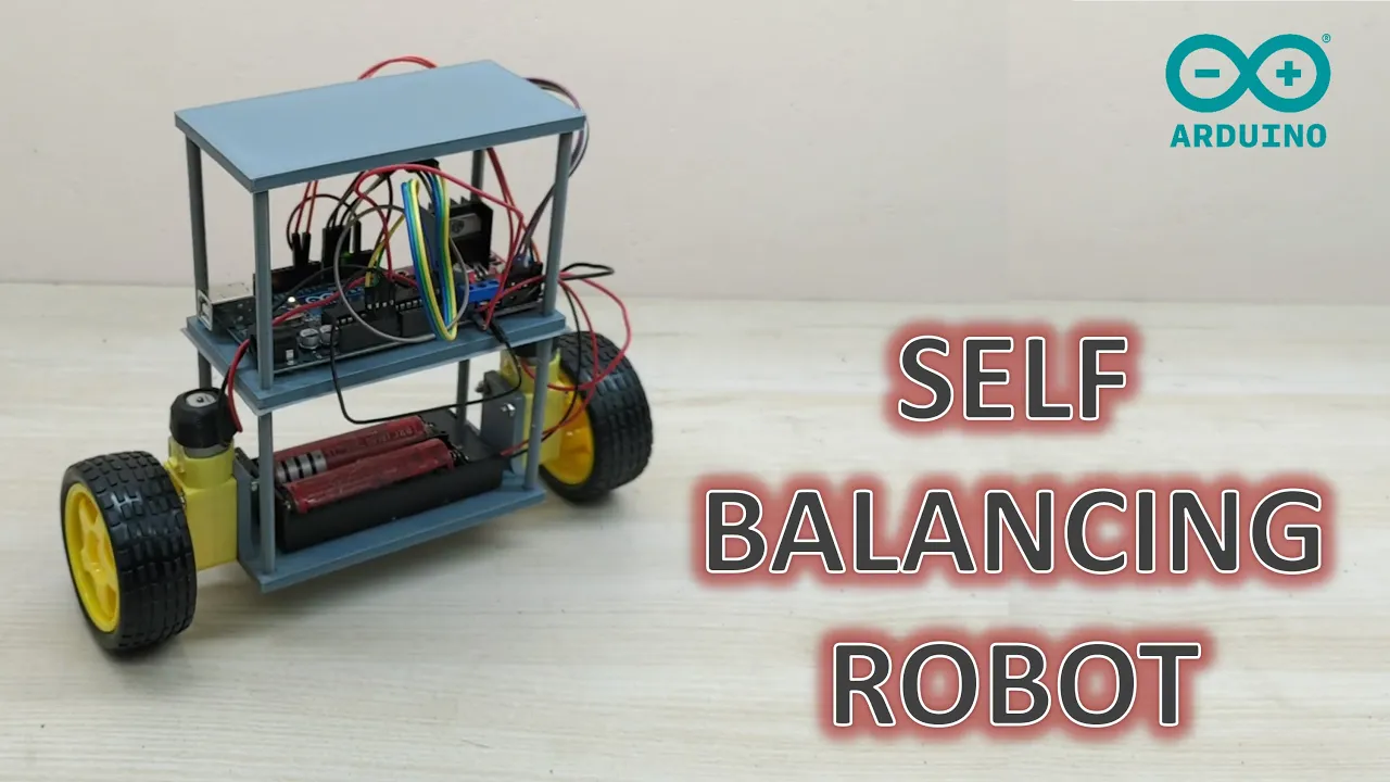
A self-balancing robot can be constructed using an Arduino Nano microcontroller, an MPU6050 accelerometer-gyroscope module for sensing tilt and rotation, a motor driver (L298N), and two BO gear motors with wheels; the robot maintains balance by continuously measuring its orientation through the MPU6050 sensor and adjusting motor speeds accordingly to counteract any tilt, allowing it to stand upright and move autonomously.
How to Build a Self-Balancing Robot: Arduino Nano & MPU6050
Added:Deep Dive
Fundamental Arduino Programming and Electronics: Familiarity with the Arduino IDE, C++ syntax, and interfacing basic components (GPIO pins, PWM, and I2C communication).

Arduino Programming Masterclass: From Basics to Libraries in 90 Mins
3.6M
Arduino is an open-source platform that enables beginners to control electronic devices using accessible programming concepts; it consists of three core components—the physical Arduino board (a microcontroller development board), the Arduino Integrated Development Environment (IDE) for writing code, and the Arduino code itself (called a sketch)—with every program requiring two essential functions: void setup() which runs once for initialization and void loop() which runs repeatedly to create continuous operation, and key functions like pinMode(), digitalWrite(), analogRead(), and analogWrite() enable interaction with inputs and outputs, while libraries provide pre-written code for complex hardware like servos and sensors, making electronics accessible to those new to programming.
Click to watch →

Proteksi Beban Lebih Arus DC, Ampere Bisa Di Atur Dengan 2 ACS712 Arduino
599
Arduino is an open-source electronics platform featuring microcontroller boards and an integrated development environment for writing C/C++ code. Key concepts include digital inputs (reading button states) and outputs (controlling LEDs), which form the foundation of interactive electronic projects. The platform enables rapid prototyping by abstracting complex hardware interactions through simple programming functions.
Click to watch →

Intro to Hardware
169
Arduino programming follows a two-part structure: setup() runs once for initialization, and loop() runs repeatedly. pinMode() configures pins as INPUT or OUTPUT. digitalWrite() sends HIGH or LOW signals to control devices. delay() creates timing intervals visible to humans. For physical circuits, LEDs require current-limiting resistors (typically 330Ω) connected between the pin and ground. The longer LED leg is the anode (positive). These fundamentals form the basis for all Arduino projects, enabling control of outputs and reading of inputs through structured code execution.
Click to watch →

PROGRAMACIÓN APLICADA A LA ELECTRONICA. CETPRO GAMOR
270
This comprehensive section covers Arduino programming and electronics fundamentals. Arduino is a free programming environment using C/C++ language. The board contains digital pins (2-13) for binary 0/1 values and analog pins (A0-A5) for continuous voltage measurements. Key hardware components include the Arduino Nano, voltage regulators (LM2596 for circuit protection), relay modules, and various sensors (PIR, magnetic, temperature, distance). Programming fundamentals include digitalWrite() for controlling outputs (HIGH/LOW) and delay() for timing. Critical rules include avoiding semicolons in library functions. The development process involves compilation (error verification) and upload to the microprocessor (AT Mega 328P). Projects demonstrate security systems, temperature monitoring, and motor control. Troubleshooting involves systematic verification using multimeters to check voltage levels and component operation. This knowledge enables students to create functional electronic projects.
Click to watch →
كيف تبرمج الأردوينو؟ وتعلم اساسيات الالكترونيات
939
Arduino is a microcontroller board that simplifies programming for electronic projects by providing built-in libraries, serial communication tools, and an intuitive IDE with setup() and loop() functions. Key concepts include understanding digital vs analog inputs, using pull-up/pull-down resistors for stable readings, implementing PWM for analog control, and interfacing with sensors like LDRs, potentiometers, ultrasonic sensors, and relays. The Arduino IDE supports various boards and libraries, making it accessible for beginners to create interactive electronic projects.
Click to watch →
Deep Dive
Understanding IMU Sensors (Accelerometers & Gyroscopes): Knowledge of how the MPU6050 measures acceleration and angular velocity, and the concept of sensor drift.

CHARLA EN VIVO, Acerca de sensores INerciales (IMU) y su uso en navegación
846
Unmanned vehicle navigation requires establishing a Cartesian coordinate system and calculating orientation angles. The Inertial Measurement Unit (IMU) consists of accelerometers and gyroscopes. Accelerometers measure acceleration and detect gravity to calculate roll and pitch angles but cannot measure yaw. They are sensitive to vibrations and rapid movements. Gyroscopes measure angular velocity in all three axes, providing 6 degrees of freedom when combined with accelerometers. However, gyroscopes suffer from drift, where small measurement errors accumulate over time, causing calculated angles to drift away from true values.
Click to watch →

How a Quadcopter Works - Flight Mechanics, Components, & Sensors (2)
95.5K
The IMU (Inertial Measurement Unit) contains two sensors: the accelerometer measures linear force exerted on the quad (linear acceleration), and the gyroscope measures rotational motion. Together, they measure linear and rotational forces but do not know the absolute position or orientation (whether the quad is upright or upside down).
Click to watch →

01 - Что такое IMU, какие бывают, основные характеристики
1.4K
IMU (Inertial Measurement Unit) is a class of semiconductor electronic devices containing mechanical components, primarily including MEMS accelerometers and gyroscopes. Accelerometers measure linear acceleration using a proof mass suspended on springs, where displacement caused by acceleration changes capacitance between movable and fixed plates, generating a digitized signal. Gyroscopes measure angular velocity by forcing a proof mass into oscillation and detecting Coriolis forces that deflect the mass when the device rotates, also using capacitive sensing. Key parameters for IMU selection include sampling frequency (typically ≥1 kHz), resolution, maximum allowable values, sensitivity, zero offset (bias), stability over time and temperature, and noise characteristics. These sensors form the basis of AHRS (Attitude and Heading Reference Systems) that process raw sensor data to provide orientation angles, with Kalman filtering used to fuse sensor data and maintain accuracy even when GPS signals are lost.
Click to watch →

Making Embedded Systems: Lesson 6.1 Introducing the sensors
1K
Inertial Measurement Units (IMUs) combine three types of sensors: accelerometers measure linear acceleration and detect orientation by sensing gravitational forces (answering 'which way is down'), gyroscopes (actually angular rate sensors) measure rotational speed around axes, and magnetometers determine direction by detecting Earth's magnetic field; these MEMS-based sensors are digital, three-axis devices prone to temperature variations and environmental interference that require calibration for accurate readings.
Click to watch →

What is an Inertial Measurement Unit (IMU)?
23.1K
An Inertial Measurement Unit (IMU) integrates three fundamental motion sensors—accelerometers, gyroscopes, and magnetometers—to enable comprehensive motion tracking. Accelerometers measure linear acceleration, detecting forces like gravity (1g when stationary) and registering zero g during free fall. Gyroscopes specialize in rotational sensing, maintaining accurate orientation measurements without human-like disorientation. Magnetometers detect magnetic fields, with compasses representing their primary navigational application for determining direction. Together, these sensors form the foundation of modern motion sensing technology, enabling features like screen orientation, heading detection, and gesture recognition through sophisticated mathematical combination.
Click to watch →
Deep Dive
Introduction to DC Motor Control: Understanding how H-bridge motor drivers and Pulse Width Modulation (PWM) are used to regulate motor speed and direction.

Aprenda a controlar motores com o Arduino! (usamos o módulo L298N)
147.8K
This section introduces DC motor control using Arduino, explaining that skills learned for controlling LEDs directly apply to motor control. The H-Bridge module (Ponte H) simplifies motor control by handling complex circuitry internally. The module has four central control pins (IN1, IN2, IN3, IN4) where each motor requires two pins: connecting one pin causes rotation in one direction, connecting the opposite pin causes reverse rotation, and connecting both or neither stops the motor. Additionally, enable pins (ENA, ENB) control whether motors are active or disabled.
Click to watch →
💡 Control de MOTORES DC con Arduino y el chip L293D 【 2021 】 - Capítulo #35🔋
137.5K
This section introduces DC motor control using the L293D H-bridge driver chip. The instructor explains that DC motors are common in toys due to their low cost and simple operation. The L293D chip enables control of both motor speed and direction, which is essential for applications like robotics. Key concepts covered include locating the chip's notch for pin identification, understanding the pin layout where pins 1-8 are counted left-to-right downward and pins 9+ right-to-left upward, and recognizing that the chip has identical configurations on both sides for controlling two motors. The instructor emphasizes never connecting motors directly to Arduino pins as this can damage the microcontroller, requiring instead an external power supply connected through the VCC and ground pins.
Click to watch →

Circuito simples que controla a velocidade de um motorzinho cc. Como Fazer!
283.1K
A simple circuit can be built to control the rotation speed of a DC motor commonly found in toy cars and CD/DVD/Blu-ray players. The circuit allows users to easily adjust how fast the motor spins.
Click to watch →

Como inverter a rotação de um motor CC, usando a ponte H mais simples do mundo.
6K
DC motors are simple to control through voltage adjustment for speed and polarity reversal for direction. While permanently reversing wires works for static applications, automatic control requires the H-bridge circuit. The simplest H-bridge uses two relays with two push buttons (CW and CCW), a DC motor, and appropriate power sources. The control circuit can use 5V while the motor uses higher voltage like 12V. This configuration allows reversible motor control for applications like conveyor belts.
Click to watch →
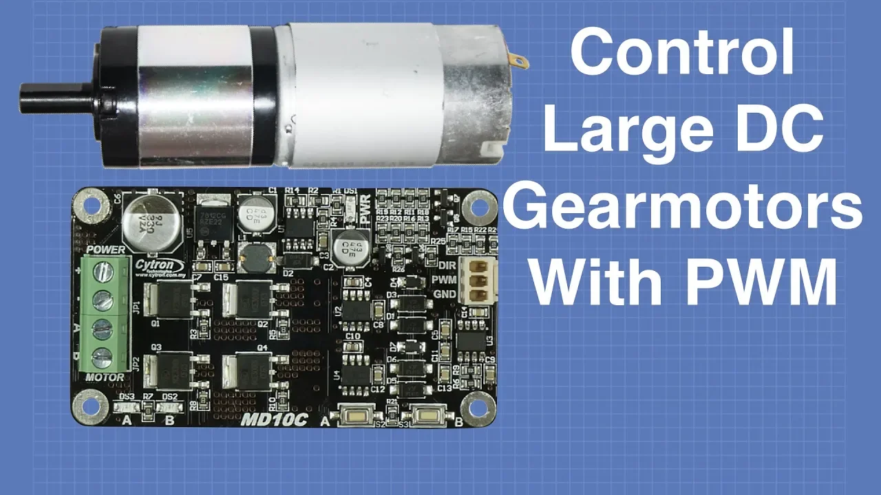
Control Large Gearmotors with PWM & Arduino
276.3K
This segment introduces DC motor control for robotics, explaining why standard motor drivers like the L298N are insufficient for large motors due to current limitations and inefficiency. The presenter covers H-bridge fundamentals, showing how four switching devices control motor direction by reversing current polarity. The key distinction between bipolar transistors (0.7V drop each, total 1.4V loss) and MOSFETs (0.1V drop each, total 0.2V loss) is explained, demonstrating why MOSFET-based controllers like the Cytron MD10C offer superior efficiency. The MD10C specifications are detailed: 5-30V operation, 13A continuous/30A peak current, no heatsink required, and 20kHz maximum PWM frequency. Practical connections are shown: Arduino ground to motor controller ground, PWM pin 3 to speed input, pin 2 to direction control, and power supply connections. The segment establishes foundational concepts for understanding advanced motor control systems.
Click to watch →
Deep Dive
Basic Feedback Control Theory (PID): Concepts of Proportional, Integral, and Derivative control loops used to adjust system outputs based on sensor feedback.

PID control explained clearly (Beginner's Guide)
970
A feedback loop continuously measures output using sensors, compares it to a set point, and makes corrections through a repeating cycle of measure, compare, and correct. PID control combines three actions: Proportional reacts to current error distance, Integral addresses accumulated error over time, and Derivative responds to rate of change. Together they reduce deviation from the set point. Proportional alone causes oscillation with overshoot and undershoot. Integral gradually eliminates steady-state error by tracking accumulated offset. Derivative anticipates overshoot by reacting to approaching changes. Modern controllers can auto-tune to optimize these parameters automatically.
Click to watch →
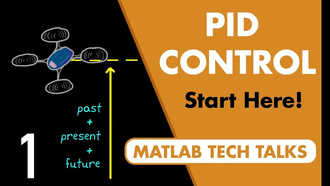
What Is PID Control? | Understanding PID Control, Part 1
2M
PID (Proportional-Integral-Derivative) control is a versatile feedback controller that uses three components to drive system error toward zero: the proportional component uses present error to generate immediate corrective action, the integral component accumulates past error over time to eliminate steady-state error, and the derivative component predicts future error based on the rate of change to prevent overshooting. This combination makes PID the most prevalent form of feedback control for physical systems because it addresses the limitations of using only proportional or integral control alone.
Click to watch →

PID Controllers | Process Control
2.7K
A feedback controller measures the control variable and uses this measurement to adjust the system. Basic components include: process, transmitter/sensor, controller, and final control element. Proper notation uses solid lines for system signals and dashed lines for electrical signals. For flammable processes, IP transducers convert electrical signals to pneumatic signals. PID controllers consist of Proportional (P), Integral (I), and Derivative (D) components. A proportional controller generates output proportional to current error: Output = Steady State + KC × Error. Key characteristics: fast response but cannot eliminate steady-state offset. Higher KC reduces offset but increases oscillation risk. The transfer function is P(s)/E(s) = KC. The controller has physical saturation limits that prevent infinite response.
Click to watch →

Pengendalian Sistem dengan Kontroler PID
357
This section covers the foundational concepts of feedback control systems and introduces PID controllers. Key topics include: (1) The three-stage process of system control: modeling (creating transfer functions), analysis (examining transient and steady-state responses), and control (implementing controllers); (2) The feedback control system structure with error signal generation (e = r - c); (3) Desired system performance characteristics: stability, good transient response (minimal overshoot, short rise and settling times), and zero steady-state error; (4) Introduction to the three basic PID control actions: proportional, integral, and derivative, which form the basis for advanced control system design.
Click to watch →

How to Thrust Vector Control | How a PID controller works and MORE control theory
34.3K
Control theory is the discipline of getting electromechanical systems to respond as intended, using feedback loops and control algorithms. A PID controller combines three components: Proportional (responds to current error), Integral (accumulates past errors over time), and Derivative (responds to rate of change). Unlike simple on/off control, PID enables nuanced responses by considering how far off a system is from its target, how long it has been off, and how quickly it is changing. Real-world applications include household thermostats maintaining temperature through continuous adjustment rather than binary switching.
Click to watch →
Prerequisite Knowledge
- Concept 01Fundamental Arduino Programming and Electronics: Familiarity with the Arduino IDE, C++ syntax, and interfacing basic components (GPIO pins, PWM, and I2C communication).
- Concept 02Understanding IMU Sensors (Accelerometers & Gyroscopes): Knowledge of how the MPU6050 measures acceleration and angular velocity, and the concept of sensor drift.
- Concept 03Introduction to DC Motor Control: Understanding how H-bridge motor drivers and Pulse Width Modulation (PWM) are used to regulate motor speed and direction.
- Concept 04Basic Feedback Control Theory (PID): Concepts of Proportional, Integral, and Derivative control loops used to adjust system outputs based on sensor feedback.
Subsequent Learning
- Step 01Advanced Sensor Fusion: Implementing Kalman Filtering or Complementary Filtering to combine accelerometer and gyroscope data for smoother, noise-resistant angle estimation.
- Step 02State-Space Control & LQR: Transitioning from traditional PID to modern control theory, such as Linear Quadratic Regulator (LQR), for more robust multi-variable stabilization.
- Step 03Wireless Telemetry and Remote Control: Integrating Bluetooth (HC-05) or Wi-Fi (ESP32) modules to remotely steer the robot and monitor its state variables in real-time.
- Step 04Autonomous Navigation and SLAM: Adding LiDAR, ultrasonic sensors, or camera systems alongside ROS (Robot Operating System) for obstacle avoidance, mapping, and path planning.
Opening Act
First Highlight
Core Segment
Climax Build
Finale Farewell
Opening Act
0:00Playing Section
- 1
Sets the stage with music and applause.
- 2
Builds initial atmosphere and engagement.
- 3
Minimal spoken content, focus on visuals.
Limitations of Basic PID and Low-Cost Hardware in Dynamic Balancing
While the Arduino Nano and MPU6050 combination is a popular, budget-friendly entry point for hobbyists, it has significant technical limitations compared to professional robotics approaches. The MPU6050 sensor is highly susceptible to noise and temperature drift, requiring complex filtering that heavily taxes the Nano's limited 8-bit processing power. Furthermore, these basic setups almost exclusively rely on classic PID (Proportional-Integral-Derivative) control. PID is a linear control strategy that struggles to manage the highly non-linear, dynamic, and unstable physics of an inverted pendulum, especially during obstacle avoidance. Robotics experts argue that for robust stability, developers should pivot to 32-bit microcontrollers (like the ESP32 or STM32) paired with advanced control methodologies like LQR (Linear Quadratic Regulator) or MPC (Model Predictive Control). These alternatives offer superior multi-variable state estimation and mathematically optimal control, which are essential for real-world reliability and complex navigation.
Deep Dive
Advanced Sensor Fusion: Implementing Kalman Filtering or Complementary Filtering to combine accelerometer and gyroscope data for smoother, noise-resistant angle estimation.

Sensör Füzyonu Nedir ? MMU Kaan 'dan Neler Beklemeliyiz ?
34.2K
This segment introduces the fundamental concepts of sensor fusion and data fusion in advanced fighter aircraft like the F-35. The discussion distinguishes between simply having advanced sensors (radar, electronic warfare systems, electro-optic cameras) and the actual capability to integrate and process data from multiple sensors into a unified operational picture. The experts explain that while fourth-generation aircraft can possess these individual sensors, the key differentiator for fifth-generation capability lies in the sophisticated data fusion algorithms that create a comprehensive situational awareness picture. The segment also addresses the proprietary nature of these algorithms, noting that specific implementation details remain classified information.
Click to watch →

Why is the F-35 the world’s most advanced fighter jet | War On Tape | Daily Mail
126.2K
Sensor fusion is the process of integrating and correlating data from multiple independent sensors—including radar, infrared cameras, electronic warfare receivers, and targeting pods—into a single unified tactical picture. Unlike fourth-generation aircraft where pilots must mentally correlate separate sensor readings, fifth-generation systems automatically fuse sensor data to identify targets, determine their type, range, and threat level, presenting this information as a single coherent track to the pilot.
Click to watch →
Turkey Getting The F-35 Is Worse Than We All Thought
18.1K
Fifth generation fighter jets like the F-35 Lightning II represent revolutionary advances in military aviation technology. The aircraft features a radar cross-section of approximately 0.00001 square meters, making it nearly invisible on enemy radar. Its AN/APG-81 radar can simultaneously track dozens of aerial targets, map ground terrain, and conduct electronic attack operations. The electronic warfare suite provides 360-degree threat awareness, while sensor fusion architecture combines data from multiple sensors into a single coherent operational picture shared across all platforms in the battle space.
Click to watch →

Modi kickstarts A REVOLUTION: Pvt Players Entry In 5th Gen Fighter Planes| Dr MJ Augustine Vinod
37.9K
Data fusion in fifth-generation fighters combines information from multiple sensors and platforms to create a comprehensive situational picture. This allows pilots to see beyond their immediate field of vision by integrating data from allied aircraft and ground stations. The system must continuously update and correct information to account for the movement of all platforms, representing a significant technological advancement. This capability transforms tactical-level fighters into strategic-level platforms, enabling detection and engagement of targets that would otherwise be invisible.
Click to watch →
US Shocked! Turkish 6th Generation Fighter Jet Is Ready For Action!
527.6K
The F-35's avionics suite represents the most sophisticated integration of military aviation technology. It includes the AAG-81 active electronically scanned array radar, AAS-239 Barracuda electronic warfare system, AAS-37 distributed aperture system, AAS-40 electro-optical targeting system, and AAS-242 communications navigation and identification suite. These systems provide rapid beam agility, multiple operational modes, all-aspect missile launch and target tracking, 10 radio frequency antennas, all-aspect radar warning receiver, self-defense against missiles, detection and jamming of hostile radars, laser targeting, forward-looking infrared capabilities, long-range IRST functions, and an unprecedented level of sensor fusion. This technology enables the pilot and friendly forces to maintain an omnipresent tactical picture of the battle space.
Click to watch →
Deep Dive
State-Space Control & LQR: Transitioning from traditional PID to modern control theory, such as Linear Quadratic Regulator (LQR), for more robust multi-variable stabilization.

State Space and LQR issues | Insight Devlog 01
4K
When implementing state space controllers like LQR (Linear Quadratic Regulator), engineers must account for real-world noise and unmodeled dynamics, as the controller's optimal gains become unstable when sensor noise or motor disturbances are present; transitioning to LQG (Linear Quadratic Gaussian) provides a more robust solution by incorporating probabilistic state estimation that handles noise through Gaussian assumptions, allowing the controller to maintain stability and achieve desired response times even in noisy environments.
Click to watch →
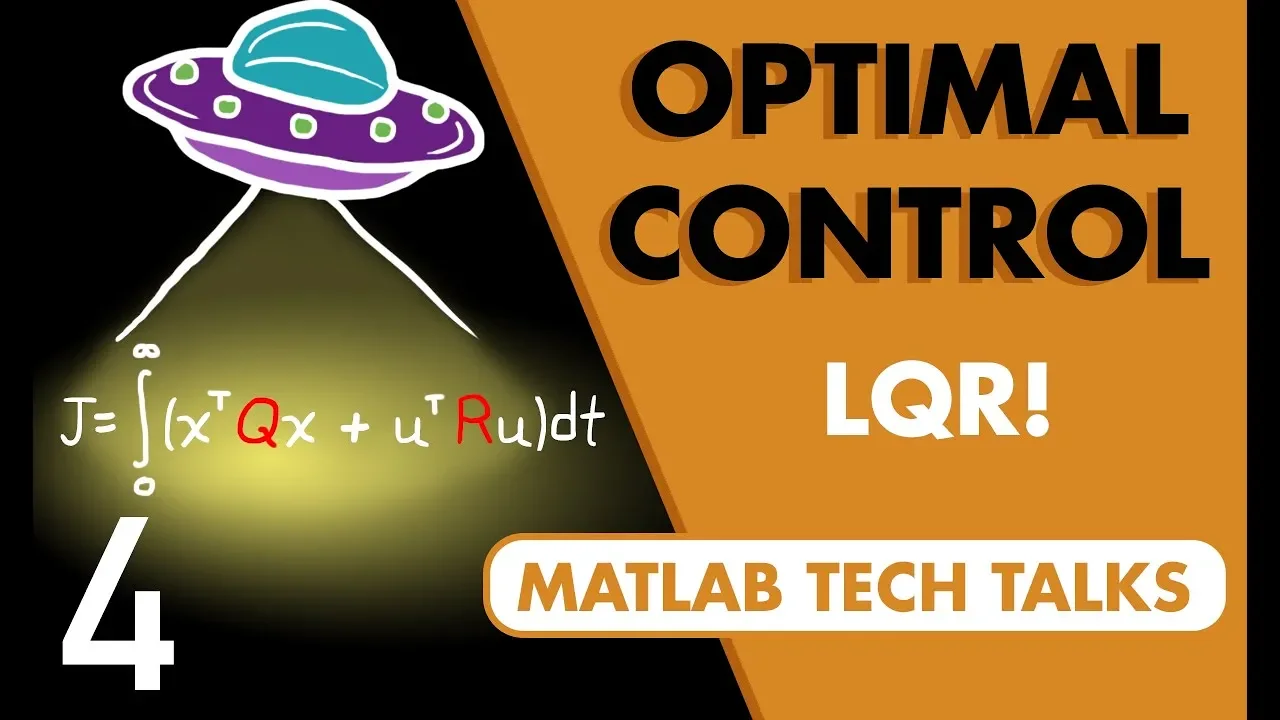
What Is Linear Quadratic Regulator (LQR) Optimal Control? | State Space, Part 4
362.1K
LQR is an optimal control methodology based on state space representation that determines the optimal gain matrix by minimizing a cost function balancing system performance and actuator effort. Unlike pole placement which directly specifies closed-loop pole locations, LQR uses mathematical optimization where designers define priorities through weighting matrices. The cost function integrates quadratic penalties on state errors and control efforts over time, ensuring convexity for a unique minimum. The Q matrix (positive definite) weights state variables to prioritize critical states, while the R matrix weights control inputs. This transforms control design from pole placement questions to intuitive tuning of performance versus effort trade-offs, making it particularly valuable for multi-input multi-output systems where manual pole placement becomes impractical.
Click to watch →
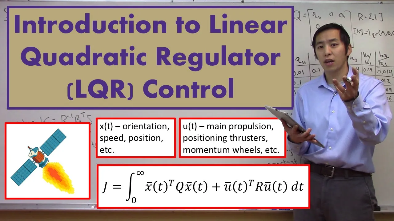
Introduction to Linear Quadratic Regulator (LQR) Control
148.5K
The optimal LQR controller is u = -Kx, where K = R⁻¹BᵀS and S satisfies the Algebraic Riccati Equation (ARE): AᵀS + SA - SBR⁻¹BᵀS + Q = 0. The design procedure involves: (1) knowing plant dynamics (A, B), (2) selecting Q and R based on requirements, (3) solving the ARE for S, (4) computing K from S, and (5) selecting the stable solution among multiple mathematical solutions. Multiple S solutions exist, requiring evaluation of closed-loop eigenvalues to identify stability. For a mass-damper system with A = [[0, 1], [-0.2, -0.2]] and B = [[0], [1]], different Q and R choices yield distinct controllers: cheap control produces aggressive gains (~10), expensive control produces conservative gains (~0.01), and partial state weighting prioritizes specific states. This mathematical framework provides the theoretical foundation for LQR controller synthesis.
Click to watch →
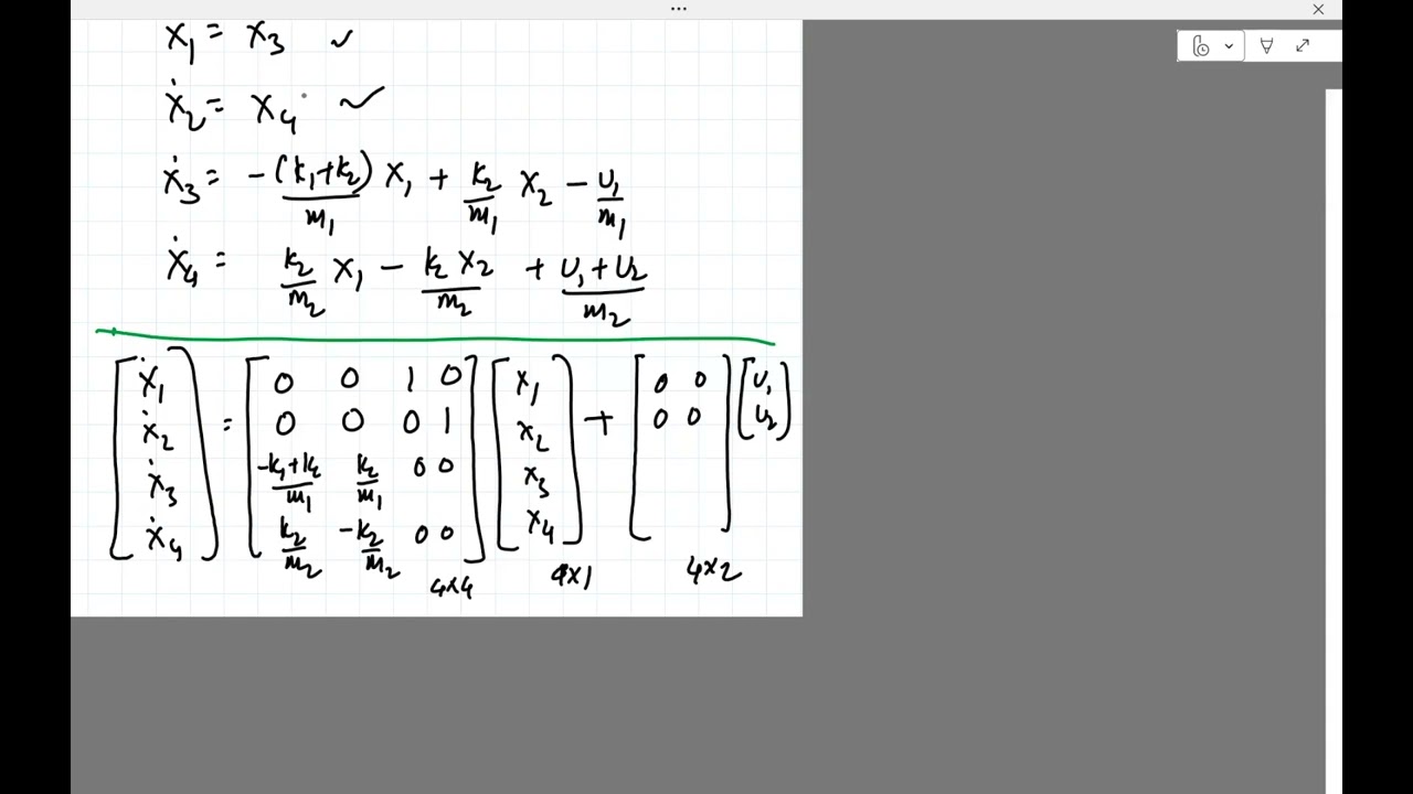
Robotics Lec18a: State space, stability, controllability, pole placement & LQR (Fall 2024)
160
The Linear Quadratic Regulator (LQR) is an optimal control method that minimizes a quadratic cost function J = ∫₀^∞ [x^T Q x + u^T R u + 2x^T N u] dt over infinite time. Here, x is the state vector, u is the control input, Q is a positive semi-definite weighting matrix for states, R is a positive definite weighting matrix for controls, and N is a cross-coupling matrix. The cost function penalizes both state deviations from zero and control effort. The matrices Q and R are user-chosen parameters that balance the trade-off between tracking accuracy and control effort. The analytical solution exists and leads to the optimal feedback gain K = -R⁻¹(B^T P + N^T), where P satisfies the Algebraic Riccati Equation.
Click to watch →
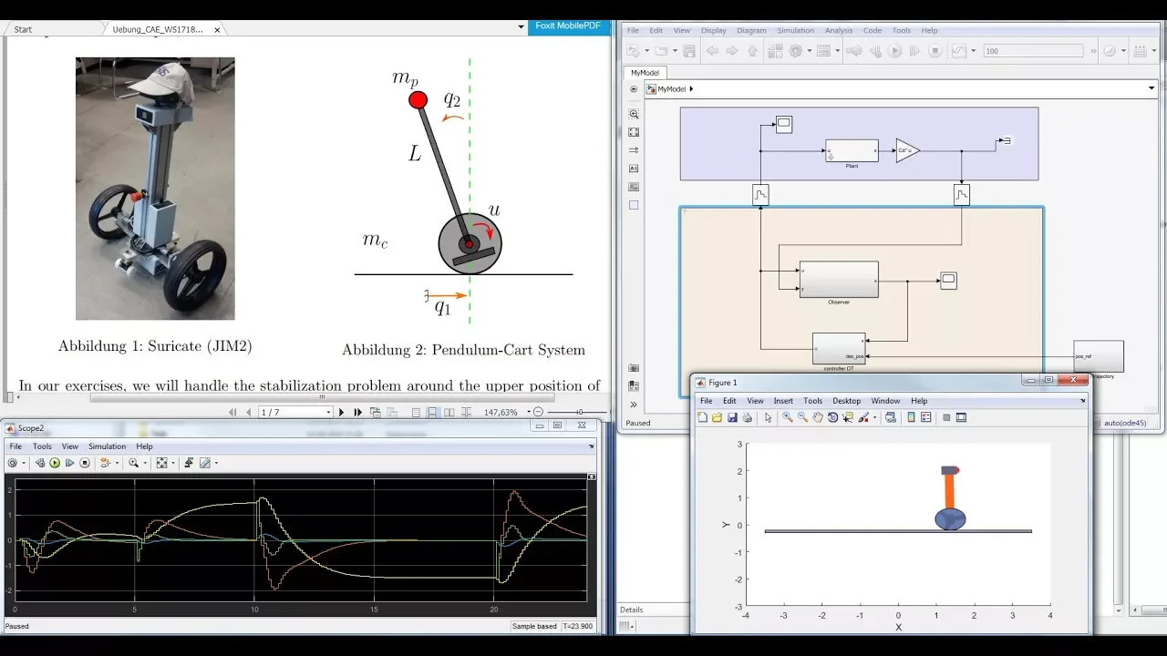
State Space Control for the Pendulum-Cart System: A short tutorial on using Matlab® and Simulink®
131.1K
LQR is an optimal control method that designs a state feedback controller by minimizing a quadratic cost function J = ∫(x^TQx + u^TRu)dt, where Q penalizes state deviations and R penalizes control effort. The controller gain K is computed using the lqr(A,B,Q,R) command. Unlike pole placement, LQR provides a systematic way to balance control performance against input effort. Increasing the weight on Q improves state regulation but increases control effort, while increasing R reduces input magnitude at the expense of slower response.
Click to watch →
Deep Dive
Wireless Telemetry and Remote Control: Integrating Bluetooth (HC-05) or Wi-Fi (ESP32) modules to remotely steer the robot and monitor its state variables in real-time.

ELPRO Training May 5 2021 905U wireless modem
2.3K
Industrial wireless radio telemetry systems enable remote monitoring and control of industrial equipment by transmitting sensor data (such as 4-20mA analog signals) over wireless networks, replacing traditional hardwired cable systems when cable installation is impractical or cost-prohibitive. These systems typically use peer-to-peer mesh networking where radios communicate directly with each other without a central master, providing redundancy and reliability. Key features include sleep mode for battery preservation, configurable update times and sensitivity thresholds, and protocol conversion capabilities that allow different control systems (like Allen Bradley and Schneider Electric) to communicate through gateway devices.
Click to watch →

Pro@ctec 2016 - Webinar 4: "Extienda su control con telemetría e instrumentación inalámbrica"
1.1K
Wireless telemetry extends control networks over long distances using radio waves instead of cables, consisting of field instrumentation (sensors/transducers), Remote Terminal Units (RTUs) for data processing and buffering, and long-range radios for communication; successful implementation requires validating communication links through link budget calculations considering transmitter power, antenna gain, cable losses, and receiver sensitivity, with antenna selection (directional vs. omnidirectional) depending on whether devices are distributed in all directions or at specific points, and system selection depends on distance requirements, data volume, real-time needs, and terrain characteristics.
Click to watch →

Wireless Wellhead - Telemetry & Remote SCADA Solutions
25.7K
Wireless wellhead telemetry systems enable remote monitoring and control of oil and gas wells through integrated wireless instrumentation, eliminating the need for complex wired infrastructure while maintaining safety certifications for hazardous environments; these systems use battery-powered controllers like the VC10 that can perform over 50,000 valve actuations and automatically retry operations when control line pressure fails to reach target levels.
Click to watch →

Введение в SCADA системы. Автоматизация производства
104.7K
Telemetry enables remote monitoring and control of distributed automation systems over communication networks. This capability allows operators to observe and manage equipment located far from the central control room, such as pipeline stations hundreds of kilometers away. Remote control functions enable operators to issue commands to field devices from centralized locations, reducing the need for on-site personnel. Telemetry systems must ensure reliable communication links, data integrity, and secure access to prevent unauthorized interference with critical infrastructure.
Click to watch →

IMPORTANT MCQ's ON TELEMETRY
1.6K
Wireless telemetry is a method of data transmission that does not require physical cables or wires. This approach enables data collection from remote or mobile locations where wired connections are impractical or impossible to implement.
Click to watch →
Deep Dive
Autonomous Navigation and SLAM: Adding LiDAR, ultrasonic sensors, or camera systems alongside ROS (Robot Operating System) for obstacle avoidance, mapping, and path planning.
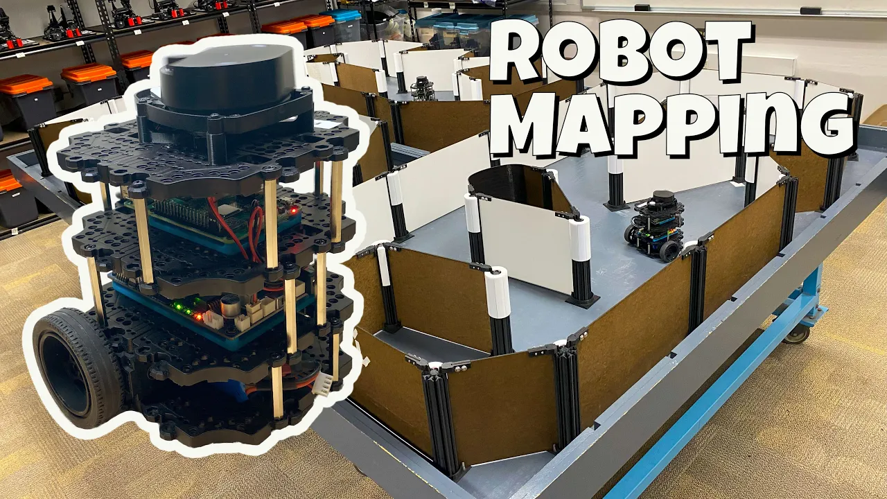
How to Make an Autonomous Mapping Robot Using SLAM
116.2K
SLAM (Simultaneous Localization and Mapping) solves the fundamental challenge where robots need both a map to navigate and accurate localization to build that map. The complete autonomous navigation pipeline involves: (1) Using LIDAR sensors to measure distances to objects by timing light reflections; (2) Creating grid-based maps where LIDAR scans fill explored areas; (3) Estimating robot position through odometry (wheel rotation measurements); (4) Correcting odometric estimates using environmental observations; (5) Identifying frontiers—boundaries between explored and unexplored areas—for systematic exploration; (6) Generating cost maps that assign wall proximity values to grid cells; (7) Finding paths that minimize distance while avoiding walls by prioritizing low-cost cells. This integrated approach enables robots to explore unknown environments autonomously.
Click to watch →

Chapter 11 SLAM and Navigation
67.5K
SLAM (Simultaneous Localization and Mapping) enables robots to create maps of unknown environments while tracking their own position within those maps. For autonomous navigation, four essential elements must work together: position sensing to determine current location, map knowledge of the operating area, path planning to calculate routes to goals, and obstacle detection to avoid collisions. The robot continuously updates its position estimate by matching sensor observations against the map, then adjusts its path as new information becomes available. This foundational framework allows robots to operate independently in unfamiliar spaces.
Click to watch →

INVENTOS LOCOS QUE TE VOLVERÁN INSANO
318.6K
SLAM (Simultaneous Localization and Mapping) is a technology that combines hardware components including Nvidia processors, LiDAR sensors, and GPS to create real-time 3D models of the environment. This technology compensates for small movements and ensures stable, safe operation even for inexperienced pilots. All collected data is stored in specialized software for convenient analysis.
Click to watch →

How I make machines see the 3D world | Daniel Cremers | TEDxTUM
12.8K
The LSD-SLAM (Large-Scale Direct SLAM) algorithm solved the SLAM problem by directly working with brightness values rather than extracted points, achieving unprecedented real-time performance. This approach maintains color consistency across camera projections without discarding brightness information. For robust autonomous navigation, multiple sensor types are fused: cameras, inertial sensors (mimicking the vestibular system), wheel odometry, and GPS. This multi-sensor fusion enables tracking precision where kilometers of driving result in only meters of drift, which GPS subsequently eliminates. This capability powers applications from autonomous robots to augmented reality and self-driving cars.
Click to watch →

Autonomous Navigation Mobile Robot using ROS | Jetson Nano | RPLidar | Differential Drive Kinematics
162.2K
Simultaneous Localization and Mapping (SLAM) enables robots to build maps while localizing themselves. The process involves launching a mapping launch file, manually driving the robot through the environment using teleop, and saving the resulting map with the map saver node. Autonomous navigation requires integrating all stack components via a launch file, providing initial pose estimates, and sending goal locations. When obstacles appear, the local planner dynamically recalculates paths, though performance may require parameter tuning. Custom Python nodes can send sequential multi-goal navigation commands, demonstrating how higher-level applications interface with the ROS navigation stack for complex autonomous behaviors.
Click to watch →
Opening Act
First Highlight
Core Segment
Climax Build
Finale Farewell
Opening Act
0:00- 1
Sets the stage with music and applause.
- 2
Builds initial atmosphere and engagement.
- 3
Minimal spoken content, focus on visuals.
Limitations of Basic PID and Low-Cost Hardware in Dynamic Balancing
While the Arduino Nano and MPU6050 combination is a popular, budget-friendly entry point for hobbyists, it has significant technical limitations compared to professional robotics approaches. The MPU6050 sensor is highly susceptible to noise and temperature drift, requiring complex filtering that heavily taxes the Nano's limited 8-bit processing power. Furthermore, these basic setups almost exclusively rely on classic PID (Proportional-Integral-Derivative) control. PID is a linear control strategy that struggles to manage the highly non-linear, dynamic, and unstable physics of an inverted pendulum, especially during obstacle avoidance. Robotics experts argue that for robust stability, developers should pivot to 32-bit microcontrollers (like the ESP32 or STM32) paired with advanced control methodologies like LQR (Linear Quadratic Regulator) or MPC (Model Predictive Control). These alternatives offer superior multi-variable state estimation and mathematically optimal control, which are essential for real-world reliability and complex navigation.
Fundamental Arduino Programming and Electronics: Familiarity with the Arduino IDE, C++ syntax, and interfacing basic components (GPIO pins, PWM, and I2C communication).
Understanding IMU Sensors (Accelerometers & Gyroscopes): Knowledge of how the MPU6050 measures acceleration and angular velocity, and the concept of sensor drift.
Introduction to DC Motor Control: Understanding how H-bridge motor drivers and Pulse Width Modulation (PWM) are used to regulate motor speed and direction.
Basic Feedback Control Theory (PID): Concepts of Proportional, Integral, and Derivative control loops used to adjust system outputs based on sensor feedback.
Advanced Sensor Fusion: Implementing Kalman Filtering or Complementary Filtering to combine accelerometer and gyroscope data for smoother, noise-resistant angle estimation.
State-Space Control & LQR: Transitioning from traditional PID to modern control theory, such as Linear Quadratic Regulator (LQR), for more robust multi-variable stabilization.
Wireless Telemetry and Remote Control: Integrating Bluetooth (HC-05) or Wi-Fi (ESP32) modules to remotely steer the robot and monitor its state variables in real-time.
Autonomous Navigation and SLAM: Adding LiDAR, ultrasonic sensors, or camera systems alongside ROS (Robot Operating System) for obstacle avoidance, mapping, and path planning.
16.8K views542likes11:04@easytechzonesOriginal Release: 2022-03-09
[Music] [Music] foreign [Music] uh [Music] [Applause] [Music] [Music] [Music] me [Music] wow [Music] so [Music] so [Music] [Music] do [Music] [Music] [Music] [Music] [Music] bye [Music] [Music] so [Music] uh [Music] you
Up Next
7:07
Self-Balancing Robot with Arduino and MPU-6050: Full Tutorial
@Science_4U_
77.9K views•2024-06-30

58:25
MathWorks Virtual RoboSub Simulation Environment | Webinar 2026
@RoboNationInc
209 views•2026-03-10

14:57
Rebuilding a Balancing Robot with Position and Velocity Control
@jamesbruton
171.9K views•2022-04-26
25:22
Micromouse: The Fastest Maze-Solving Robots on Earth
@veritasium
23.5M views•2023-05-24
Related Study Plans & Knowledge Roadmaps
Structured learning paths in Robotics
robotics
Building Delta Robots: Kinematics & Pico
01Foundations of Delta Robots & Mechanical Design
02Electronics and Microcontroller Setup with Pi Pico
03Delta Robot Kinematics and Coordinate Math
+ 3 more learning modules
65h6 modules
Explore Roadmap
robotics
Building Ballbots: Dynamics, Kalman & LQR
01Embedded Electronics & Omniwheel Actuation
02Ballbot Kinematics & Rigid Body Dynamics
03IMU Sensors & Kalman Filter State Estimation
+ 2 more learning modules
42h5 modules
Explore Roadmap
robotics
Micromouse: Hardware, PID Control & Flood-Fill
01Electronics & Teensy Microcontroller Basics
02Sensors and Actuators: Motors, Encoders & IR
03Precision Movement: Implementing PID Control
+ 2 more learning modules
35h5 modules
Explore Roadmap
robotics
CDPR: Kinematics, Arduino & Winch Control
01Foundations of Arduino & Basic Electronics
02Stepper Motors and Winch Mechanics
03Kinematics of 2D Cable-Driven Robots
+ 2 more learning modules
28h5 modules
Explore Roadmap