This tutorial demonstrates how to convert depth maps into 3D point clouds using Open3D library by processing RGB and depth images through image flipping, color format conversion, and array transformation, then creating an RGBD image using Open3D's CreateFromColorAndDepth function, and finally generating the point cloud with PointCloudFromRGBD function while applying camera intrinsic parameters for accurate depth representation.
Depth Map to Point Cloud Conversion Using Open3D and Python
Added:Deep Dive
Basic Python programming, including familiarity with scientific computing libraries like NumPy.

4.1 Intro to NumPy (L04: Scientific Computing in Python)
13.9K
NumPy is a fundamental Python library for scientific computing that provides efficient array operations through contiguous memory storage and optimized C/C++ implementations, making it significantly faster (e.g., 100x speedup for dot products) than native Python lists; it serves as the foundation for most Python scientific computing libraries including SciPy, Pandas, and scikit-learn, and implements n-dimensional arrays (ndarray) with fixed data types and dimensions that enable efficient mathematical computations and data manipulation.
Click to watch →

🐍Python for Beginners: Learn Python in 7 Hours Step-by-Step in Tamil | kaashiv infotech reviews
52.3K
NumPy is a fundamental Python library for numerical computing, providing support for large multi-dimensional arrays and matrices. It includes functions for mathematical operations, random number generation, and linear algebra operations. NumPy arrays (ndarrays) are more efficient than Python lists for numerical computations due to homogeneous data storage and optimized C-based implementations. The library serves as the foundation for many other scientific computing libraries in Python, including Pandas, SciPy, and scikit-learn.
Click to watch →

NumPy Beginner | SciPy 2016 Tutorial | Alexandre Chabot LeClerc
106.6K
Numpy forms the foundational layer of Python's scientific computing stack, providing two core capabilities: (1) ND arrays (n-dimensional arrays) that enable efficient memory storage and fast numerical computations, and (2) Universal Functions (ufuncs) that perform vectorized operations like addition, subtraction, multiplication, and mathematical functions on entire arrays without explicit Python loops. Originally designed to offer MATLAB-like capabilities within Python, Numpy has evolved into a mature project with over 400 contributors and millions of downloads monthly. It serves as the basis for higher-level libraries like SciPy and integrates seamlessly with other scientific tools.
Click to watch →

Python-based scientific computing I
7.7K
Python is an excellent language for scientific computing due to its readability, high-level abstraction, and extensive scientific libraries (NumPy, SciPy, Matplotlib). Key concepts include: variables are references to objects (not containers), so assignment creates references rather than copies; lists are mutable sequences supporting slicing and efficient appending, while tuples are immutable; dictionaries provide O(1) key-value lookups; control flow uses indentation-based blocks; and functions are first-class objects that can be passed around. The scientific Python ecosystem enables rapid development and exploration, with development time being more important than raw CPU speed for most scientific applications.
Click to watch →
![ปูพื้นฐานการใช้ Python ร่วมกับ NumPy | สำหรับงาน Data Science [FULL COURSE]](https://i.ytimg.com/vi/MDA8SbfdLKA/hqdefault.jpg)
ปูพื้นฐานการใช้ Python ร่วมกับ NumPy | สำหรับงาน Data Science [FULL COURSE]
101K
NumPy is a fundamental Python library for mathematical calculations and data management in scientific computing, statistics, and engineering. It provides efficient array operations that are essential for data science workflows. The library enables fast numerical computations that would be slow with standard Python lists. Understanding NumPy is crucial for anyone working with data analysis, machine learning, or scientific computing in Python.
Click to watch →
Deep Dive
Fundamentals of computer vision, specifically the pinhole camera model and lens distortion.

Week 3: Computer Vision | NPTEL noc25-cs143 Full Discussion
641
Camera geometry defines the mathematical relationship between 3D real-world points and their 2D projections on the image plane. The pinhole camera is the simplest model with three key properties: a single camera center through which all light rays pass, a flat image plane where rays intersect to form images, and no lens distortion. The coordinate system includes the camera center C, principal plane (containing C), principal axis (Z-axis), principal point O (intersection of principal axis with image plane), and focal length f (distance from C to O). The projection formula x = f*X/Z and y = f*Y/Z is derived from similar triangles, showing how 3D coordinates map to 2D image coordinates.
Click to watch →
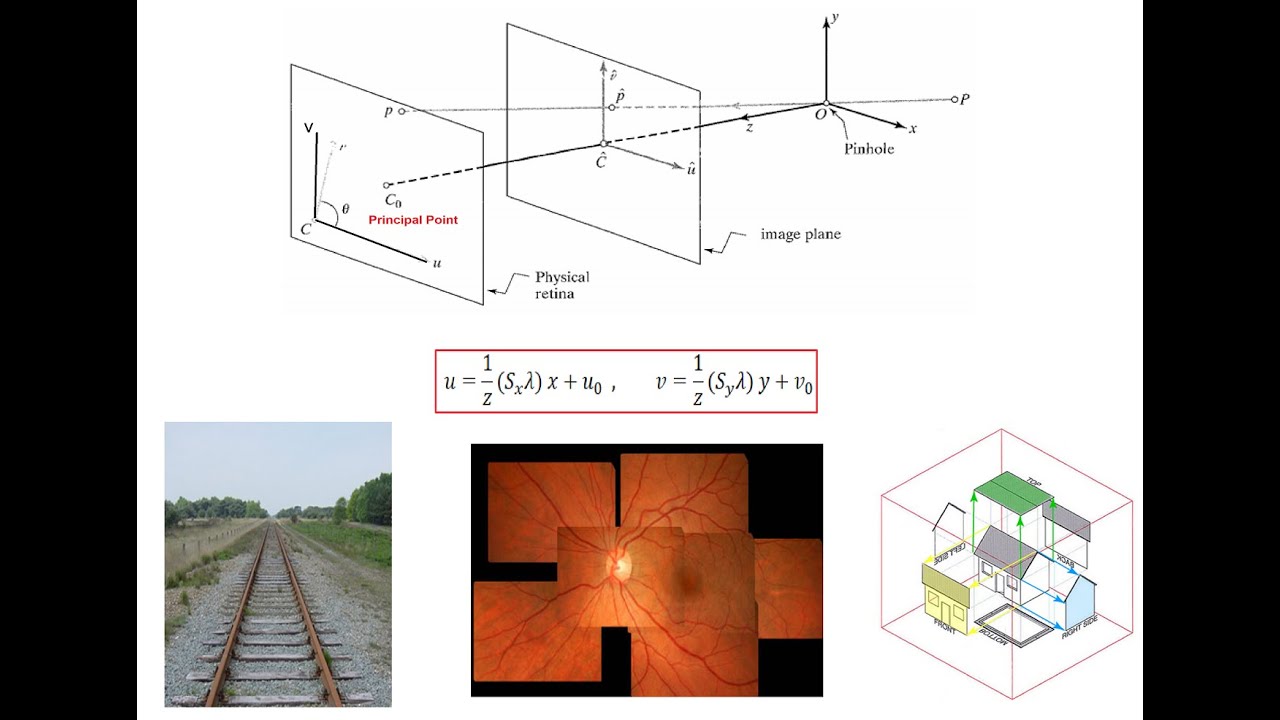
Pinhole Camera Model, Perspective, Affine and Orthographic Projections
5.6K
Computer vision is the science and technology of machines that see, utilizing cameras and sensors to extract meaningful information from visual data. Image processing involves computational manipulation of digital images, while computer vision extracts higher-level semantic meanings. Every computer vision system must be independently tuned for its specific application and goals—there is no universal 'one-size-fits-all' solution. The pinhole camera model is the simplest and most widely used mathematical representation of camera projection, where light rays from scene points pass through a single pinhole before hitting an image plane at distance λ (focal length) behind it. This creates an inverted image where distant objects appear smaller than closer objects of the same actual size, and parallel lines converge toward vanishing points on the horizon line.
Click to watch →

CVFX Lecture 17: Image formation and single-camera calibration
70.9K
The pinhole camera model describes basic image formation: light passes through a small aperture and projects an inverted image onto a film or sensor plane behind it. In computer vision, we often assume the image plane sits in front of the camera center for convenience, avoiding the inversion. The distance between the camera center and the image plane is called the focal length (f). This model forms the foundation for understanding how 3D world points project to 2D image coordinates.
Click to watch →

Lecture 1: Introduction to Machine Vision
109.4K
The pinhole camera model establishes fundamental relationships between 3D world coordinates and 2D image coordinates using similar triangles: x/f = X/Z and y/f = Y/Z. This camera-centric coordinate system places the center of projection at origin with optical axis aligned to Z-axis, simplifying mathematics. Vector notation compactly expresses these relationships, though differentiation reveals nonlinear dependencies on depth. The model shows why perspective projection is nonlinear (division by Z) yet exploitable: depth information can be recovered by analyzing how image positions change. This mathematical framework enables subsequent analysis of motion, calibration, and optimization methods throughout the course.
Click to watch →

The Camera Transform
134.1K
The camera transform is the standard method in computer graphics for placing a camera in 3D space and projecting it into an image. Developed in the late 1970s and early 1980s, it models everything on a pinhole camera basis where light rays enter obliquely through a small hole. The challenge with pinhole cameras is that oblique rays require complex mathematical calculations. Computer graphics uses parallel projection onto a plane as a more efficient alternative, where the Z coordinate is simply forgotten and only X and Y are used for projection. Perspective projection creates the visual effect where objects farther away appear smaller and objects closer appear larger, achieved through an inverse relationship with depth (Z coordinate). The fourth coordinate (W) in the transformation matrix becomes similar to Z, and dividing by W during perspective division creates the perspective effect.
Click to watch →
Deep Dive
Understanding of camera intrinsic parameters (focal length, principal point) and coordinate systems.

CSE 565 spring 2022 03 07
266
Real camera systems have several intrinsic parameters: focal length f, pixel dimensions (k for width, l for height), and the principal point (u0, v0) which is the origin of the image coordinate system. The image coordinates are measured in pixels (rows and columns), while physical coordinates are in millimeters. The skew angle θ represents the angle between the u and v axes, which may not be exactly 90 degrees in real cameras. These parameters relate the physical 3D world to the discrete image sensor, enabling accurate camera modeling and 3D reconstruction.
Click to watch →
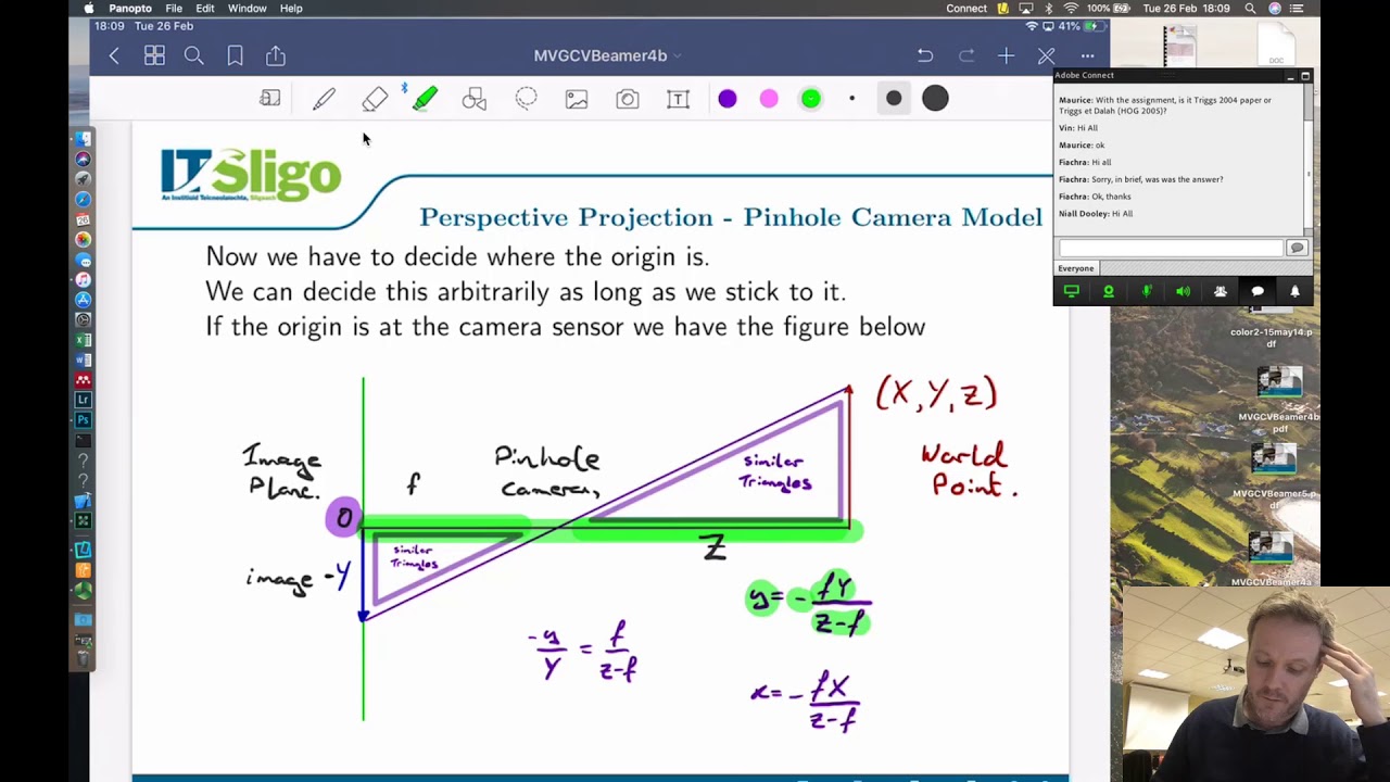
Lecture 4B Modelling the Camera
1.4K
Camera intrinsic parameters describe the internal geometry of the camera and include: focal length (f), principal point (cx, cy) which is the center of the image sensor, and pixel scale factors (sx, sy) that convert continuous coordinates to discrete pixel coordinates. These parameters are typically combined into a 3×3 matrix called the camera matrix K. The intrinsic parameters determine how 3D points are projected onto the 2D image plane.
Click to watch →
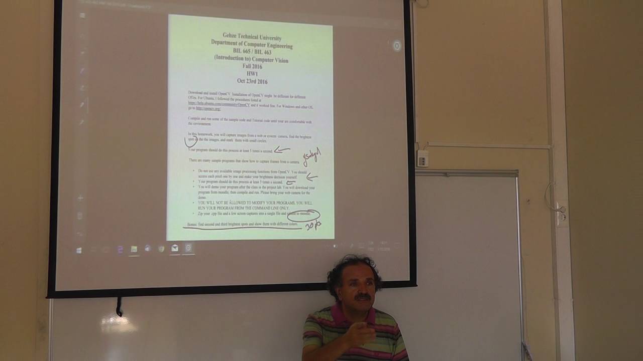
2016 Fall GTU CSE 665 Oct 03 Lecture 03 00000
208
The instructor explains camera intrinsic parameters (focal length, skew coefficient, principal point) that define how the camera projects 3D points to 2D image coordinates. These parameters are embedded in a 3x3 matrix and remain constant for a given camera regardless of position. Extrinsic parameters (rotation and translation) describe the camera's position and orientation in the world coordinate system and change when the camera moves. The complete projection matrix combines both intrinsic and extrinsic parameters to transform world coordinates to image coordinates.
Click to watch →
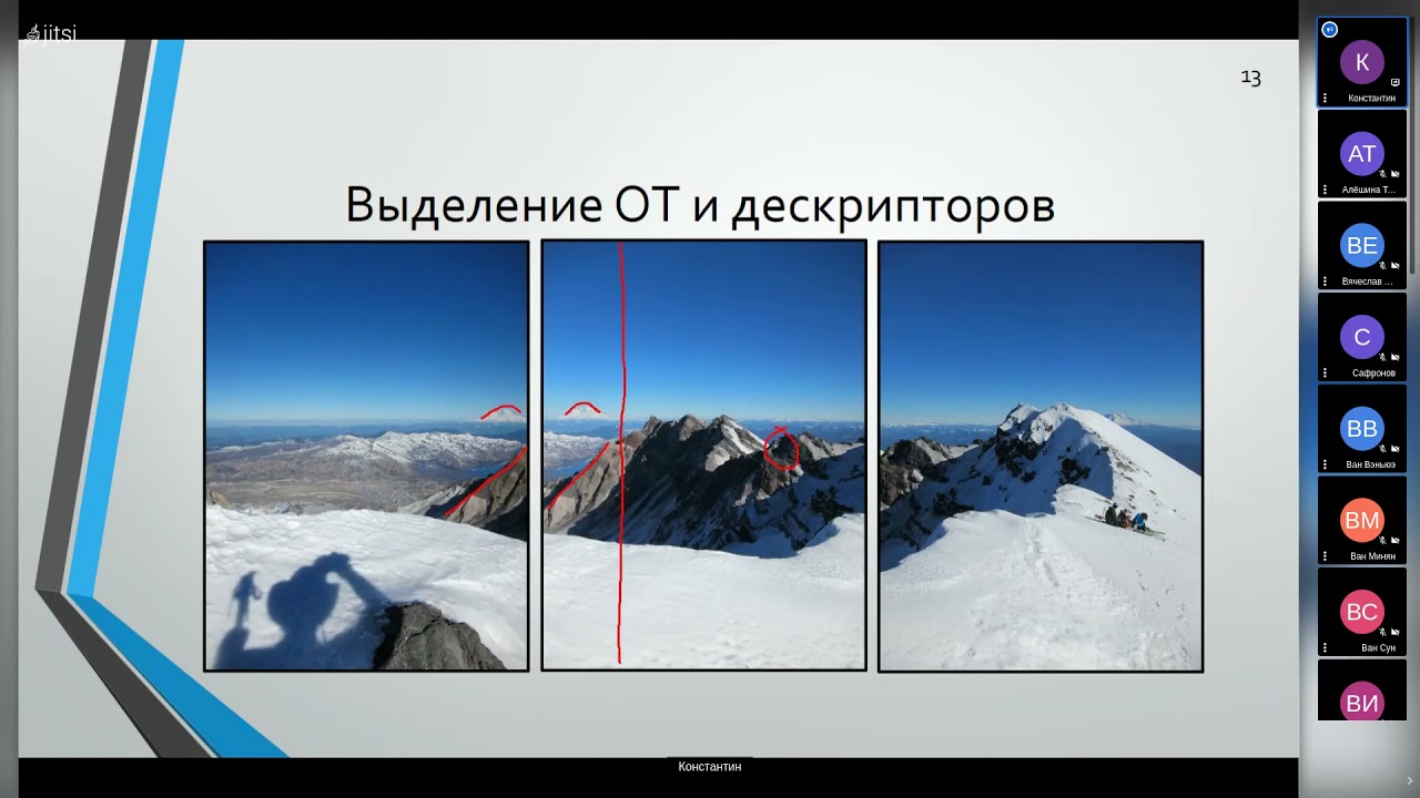
Лекция 7 Введение в компьютерное зрение
549
Camera parameters include: (1) focal length - the distance from the lens to the image plane, which determines the field of view, (2) principal point - the center of the image where the optical axis intersects, (3) skew - the angle between the image axes, and (4) pixel dimensions. These parameters are essential for accurate camera calibration and for converting between 3D world coordinates and 2D image coordinates. The coordinate system typically has the origin at the top-left corner of the image, with x increasing to the right and y increasing downward.
Click to watch →
![[Introduction to Computer Vision] 4. Camera Calibration](https://i.ytimg.com/vi_webp/rHYFqx87wvE/maxresdefault.webp)
[Introduction to Computer Vision] 4. Camera Calibration
158
Intrinsic camera parameters describe the internal characteristics of the camera, including focal length (focal length in X and Y directions) and principal points (image center). These parameters define how the 3D camera coordinate system projects to the 2D image coordinate system. Extrinsic camera parameters describe the camera's position and orientation in the world, including 3D rotation and 3D translation. These parameters define the transformation from the 3D world coordinate system to the 3D camera coordinate system.
Click to watch →
Deep Dive
The concept of depth images/maps and how they store spatial distance information per pixel.
3D Scanning & Motion Capture: 1. 3DConcepts
6.3K
A depth image stores the distance from the camera to each pixel on a per-pixel basis, in addition to color information. The depth values are typically stored as z-coordinates in the camera's coordinate frame (the viewing direction). The camera frame has x, y, z axes where z points into the viewing direction. Depth images can be visualized using HSB color mapping where different colors represent different distances, or as grayscale images.
Click to watch →

제3의 눈! 3D 카메라 혁명! 과연 현재 기술은 어디까지 와있을까? 3D 카메라 1부! (딥인사이트 오은송 대표)
19.8K
Depth data, also called depth maps, is the information that shows the distance of objects from the camera at each pixel location. In a 2D image, you can see that someone is wearing a suit, but you cannot determine whether they are close or far away. Depth data provides this crucial spatial information, enabling systems to understand the 3D structure of their environment and make decisions based on object positions and distances.
Click to watch →

11월 알쓸유잡 : 우리 인생에는 그림자가 없기를 - 그림자 구현에 대한 이해
7.7K
A depth map is a render target that stores depth information (distance values) from a camera to every pixel in the scene. Each pixel in the depth map contains the distance from the camera to the nearest surface at that position. This depth information is fundamental for determining occlusion relationships between objects and is used by hardware to process visibility and occlusion efficiently.
Click to watch →
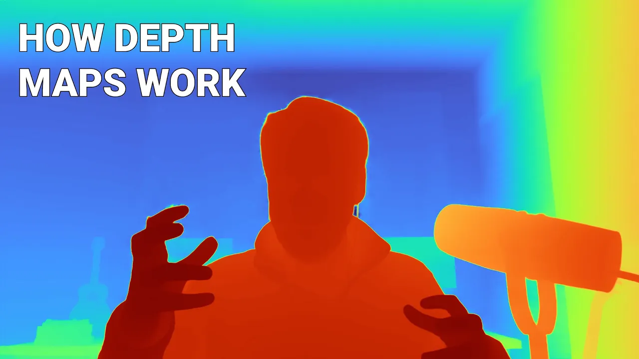
Exploring Depth Maps in Computer Vision
2.8K
Depth in computer vision refers to the distance of objects from a reference point, measured in units like meters or feet. A depth map is a 2D grid where each pixel stores depth information instead of color, enabling spatial understanding of environments. Depth data can be stored in RGB-D formats combining color and depth or separated for specialized applications. Different sensors produce different representations: laser scanners create point clouds with XYZ coordinates, while volumetric representations like voxels and octrees model depth throughout 3D spaces. The choice of representation depends on the application requirements and sensor capabilities.
Click to watch →
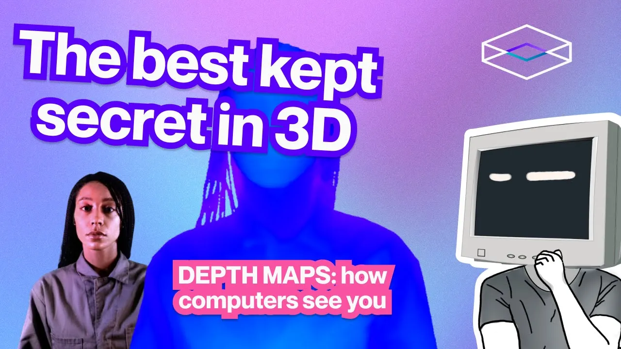
What are depth maps (and why should you care)?
4K
A depth map is a 2D image where each pixel contains distance information from a reference point (like a camera), enabling computers to perceive depth and create realistic 3D effects; this technology powers applications ranging from self-driving cars and medical imaging to smartphone portrait mode and 3D gaming, allowing devices to understand spatial relationships that humans naturally perceive through stereoscopic vision.
Click to watch →
Prerequisite Knowledge
- Concept 01Basic Python programming, including familiarity with scientific computing libraries like NumPy.
- Concept 02Fundamentals of computer vision, specifically the pinhole camera model and lens distortion.
- Concept 03Understanding of camera intrinsic parameters (focal length, principal point) and coordinate systems.
- Concept 04The concept of depth images/maps and how they store spatial distance information per pixel.
Subsequent Learning
- Step 01Point cloud preprocessing operations, such as voxel downsampling, outlier removal, and normal estimation.
- Step 02Point cloud registration techniques (e.g., Iterative Closest Point - ICP) to align and merge multiple 3D scans.
- Step 033D surface reconstruction methods (e.g., Poisson or Ball Pivoting algorithms) to convert point clouds into solid 3D meshes.
- Step 04Integrating 3D point cloud data into deep learning pipelines for object detection, segmentation, or classification (e.g., PointNet).
Point Cloud Creation
Laparoscopic Application
Point Cloud Creation
0:00Playing Section
- 1
Generates 3D point cloud from depth and RGB images using Open3D.
- 2
Converts images, sets camera intrinsics, and creates RGBD data.
- 3
Displays point cloud with adjustable view control for inspection.
Volumetric TSDF Fusion and Implicit Representations over Raw Point Clouds
While converting depth maps to raw point clouds using Python and Open3D is a standard geometric approach, it has significant limitations. Raw point clouds are discrete, unstructured, and highly sensitive to sensor noise and occlusions, making them inefficient for downstream tasks like rendering, physics simulation, or precise 3D reconstruction. A major alternative perspective advocates for volumetric integration methods, such as Truncated Signed Distance Field (TSDF) fusion, or modern implicit representations like Neural Radiance Fields (NeRFs) and 3D Gaussian Splatting. Instead of generating isolated 3D points, these methods fuse depth data into a continuous volumetric grid or neural field. This mathematical formulation naturally filters out sensor noise, resolves overlapping geometries, and directly generates closed, watertight meshes. Furthermore, for real-time applications like robotics, Python-based CPU processing introduces performance bottlenecks, leading industry practitioners to favor GPU-accelerated frameworks (e.g., PyTorch3D) or highly optimized C++ libraries (such as PCL) over standard Open3D Python implementations.
Deep Dive
Point cloud preprocessing operations, such as voxel downsampling, outlier removal, and normal estimation.

Point Clouds on the Go: How to Create 3D Models with Your Phone
12.6K
This comprehensive tutorial demonstrates creating 3D point clouds from smartphone videos through a complete workflow: (1) Capture panoramic video with varied viewpoints and sufficient motion; (2) Convert video to individual TIFF frames using editing software or online converters; (3) Import frames into photogrammetry software like Agisoft Metashape; (4) Align photos by detecting matching features and estimating camera positions; (5) Generate dense point cloud with configurable quality settings; (6) Export point cloud in standard formats (PCD/Ply); (7) Load into Open3D for advanced processing including voxel downsampling, normal estimation, and outlier removal. The process transforms raw video footage into structured 3D geometric data suitable for various applications.
Click to watch →
![[3D Point Cloud Data Processing]Chapter 6.Pointcloud Analysis #1: Filtering, Nearest Neighbor Search](https://i.ytimg.com/vi_webp/mQAJyrh3Bfg/maxresdefault.webp)
[3D Point Cloud Data Processing]Chapter 6.Pointcloud Analysis #1: Filtering, Nearest Neighbor Search
1.3K
Point cloud filtering involves downsampling (reducing point density for faster processing) through methods like Voxel Grid, Farthest Point Sampling (FPS), and Normal Space Sampling (NSS), and noise removal using Radius Outlier Removal and Statistical Outlier Removal. Nearest neighbor search employs KD-Tree and Octree data structures to efficiently find k-nearest neighbors or radius-based neighbors in 3D point clouds, with KD-Tree partitioning space using hyperplanes and Octree dividing space into octants.
Click to watch →
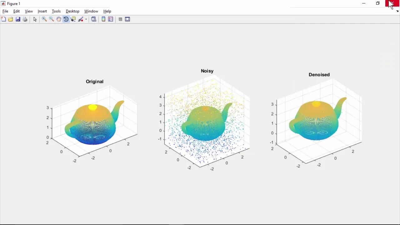
Point Clouds | Student Competition: Computer Vision Training
22.7K
Point clouds are large collections of XYZ coordinate points representing 3D object surfaces, created by LiDAR and stereo cameras. Data is stored in PLY/Stanford triangle format with each point as a separate line. In MATLAB, PC read loads ply files into point cloud objects with properties for coordinates, point count, and axis limits. Visualization uses PC show (default Z-axis up) or PC player (100x faster for streaming data with automatic downsampling). Data pre-processing is essential due to gigabyte-scale datasets. Down sampling reduces data using three methods: Random (fastest, random selection), Box grid/grid average (merges points in uniform 3D boxes to preserve shape), and Non-uniform box grid (creates boxes with equal points to preserve relative density best). Denoising uses PC denoise with num_neighbors (controls sensitivity) and outlier threshold (removes points with high average neighbor distance). Trade-offs exist between computational speed and quality preservation.
Click to watch →

SCAN to BIM for Bridges: Extraction of Geometric Properties for Engineering Analysis - Tina Agbor
215
This video presents a comprehensive workflow for converting bridge point cloud data into BIM models for engineering analysis, involving point cloud preprocessing (noise removal using statistical outlier detection, downsampling with voxel methods, and normal estimation), segmentation using Z-planes to separate structural components like spandrel walls, piers, and rings, mesh generation using alpha shapes, and automated BIM model creation in Revit with parameter extraction for geometric properties including height, width, span, and thickness measurements.
Click to watch →

Houdini 20 Lidar tools
6.9K
Effective LiDAR processing requires systematic preprocessing before mesh generation. The Point Cloud Reduce node reduces computational load by sampling points within defined box sizes, with larger boxes producing fewer points. Sample methods include averaging near centers or random selection. The Point Cloud Normal node calculates surface normals essential for meshing, offering two methods: Local propagation for general cases and Orient normals towards hint for large-scale terrain where consistent upward orientation is desired. Proximity radius and neighborhood parameters control how many neighboring points influence each normal calculation, requiring adjustment based on terrain scale.
Click to watch →
Deep Dive
Point cloud registration techniques (e.g., Iterative Closest Point - ICP) to align and merge multiple 3D scans.

Gentle Introduction to Point Cloud Registration using Open3D
6.1K
Point cloud registration aligns multiple fragmented scans into a unified coordinate system, with Iterative Closest Point (ICP) being the most popular method that iteratively transforms one cloud to match another through translation and rotation; ICP has two variants—point-to-point which minimizes squared Euclidean distances between corresponding points, and point-to-plane which additionally considers surface normal information by projecting error vectors onto normals via dot product—where the choice between them depends on the specific application requirements; importantly, effective registration follows a two-stage workflow where global registration provides an approximate initial alignment to avoid local minima, followed by local registration methods like ICP for fine-tuning to achieve precise alignment.
Click to watch →

CLOUDCOMPARE TUTORIAL FROM POINT CLOUD TO MESH AND RENDERING VIEWS.
298
Point cloud alignment involves matching multiple scans to a common coordinate system. The align command uses reference points (minimum 4) that are visible in both clouds, with distributed points improving accuracy. RMS (Root Mean Square) below 0.02 indicates good alignment. ICP (Iterative Closest Point) automatically registers clouds by minimizing distances between all points. Global RMS analysis validates alignment quality across all points, identifying regions with poor capture quality.
Click to watch →

Week 9: Computer Vision | NPTEL noc25-cs143 Full Discussion
284
Registration aligns multiple range images of the same object into a common coordinate system. Since single viewpoints cover only partial objects, multiple scans are needed. The rigid transformation is P_B = R × P_A + T, where R is rotation, T is translation. The goal minimizes error between corresponding points. The Iterative Closest Point (ICP) algorithm: initialize R,T; compute error; refine parameters; repeat until convergence. ICP is computationally efficient and widely used for 3D reconstruction, though it requires good initial alignment. This enables complete 3D shape reconstruction from partial scans.
Click to watch →
LiDAR Point Set Registration
405
Point set registration (scan matching) computes the rigid spatial transformation (translation x,y + rotation theta) that aligns a source point cloud with a target point cloud. The process requires data association - finding correspondences between source and target points, often using nearest-neighbor heuristics when no prior information exists. The Iterative Closest Point (ICP) algorithm implements this through three iterative steps: (1) associate source points with their closest target neighbors, (2) define an error function measuring misalignment, (3) minimize this error through iteration. This enables self-localization by comparing new scans against a reference map and accumulating transformations over time.
Click to watch →

Iterative Closest Point (ICP) - Computerphile
151.6K
The Iterative Closest Point (ICP) algorithm is a popular method for aligning point clouds by iteratively finding correspondences between points in two sets and optimizing the translation and rotation to minimize distances between matched points, though it may converge to local minima if initial estimates are poor.
Click to watch →
Deep Dive
3D surface reconstruction methods (e.g., Poisson or Ball Pivoting algorithms) to convert point clouds into solid 3D meshes.
How to Turn/Scan Objects Into 3D Models With Just a Camera
264.2K
Surface reconstruction converts point clouds into watertight meshes. Two primary methods: Poisson reconstruction (faster, preferred for most cases) and Floating Scale Surface Reconstruction (slower, more detailed). Poisson uses depth parameters (8-9 recommended) and produces clean results with minimal artifacts. Floating Scale offers higher detail but generates more artifacts around complex features. Confidence thresholds and minimum component sizes help reduce unwanted artifacts. For CMVS/PMVS, unchecking visibility information improves results with smaller photo sets. Default settings often produce the best balance of quality and performance.
Click to watch →

05 - Surface Reconstruction from 3D Point Cloud
144
This video explains how to convert raw 3D point clouds into continuous mesh representations using four key algorithms: Convex Hull (smallest convex shape containing all points, good for bounding volumes), Alpha Shape (generalized convex hull controlled by alpha parameter to capture concavities), Ball Pivoting Algorithm (rolls virtual ball across points to form triangles), and Poisson Surface Reconstruction (solves Poisson equation for smooth, watertight surfaces). Normal estimation via PCA is essential for BPA and Poisson methods. These techniques are fundamental in LiDAR processing, medical imaging, game asset creation, and robotics.
Click to watch →
3D scanning with Photogrammetry for free! - Tutorial
802.8K
Apply the Surface Reconstruction Poisson filter under Filters > Point Set to convert the point cloud into a solid mesh. Recommended parameters are typically 12 for the first value, 7 for the second, and 1 for the remaining parameters. This algorithm generates a watertight surface from the point cloud data. If the result has issues, delete the problematic mesh and reapply the filter with adjusted parameters. The process may require multiple iterations to achieve optimal results.
Click to watch →
Meshlab - Crea una mesh da una nuvola di punti
8.1K
MeshLab's Poisson surface reconstruction algorithm converts point cloud data into 3D meshes by decomposing the point cloud into progressively smaller packets to create a detailed surface; the reconstruction depth parameter controls mesh detail (higher values like 10-14 produce richer meshes but require more processing time), with the software offering various visualization options including wireframe, solid, and point cloud views, along with mesh editing tools for vertex and face manipulation.
Click to watch →
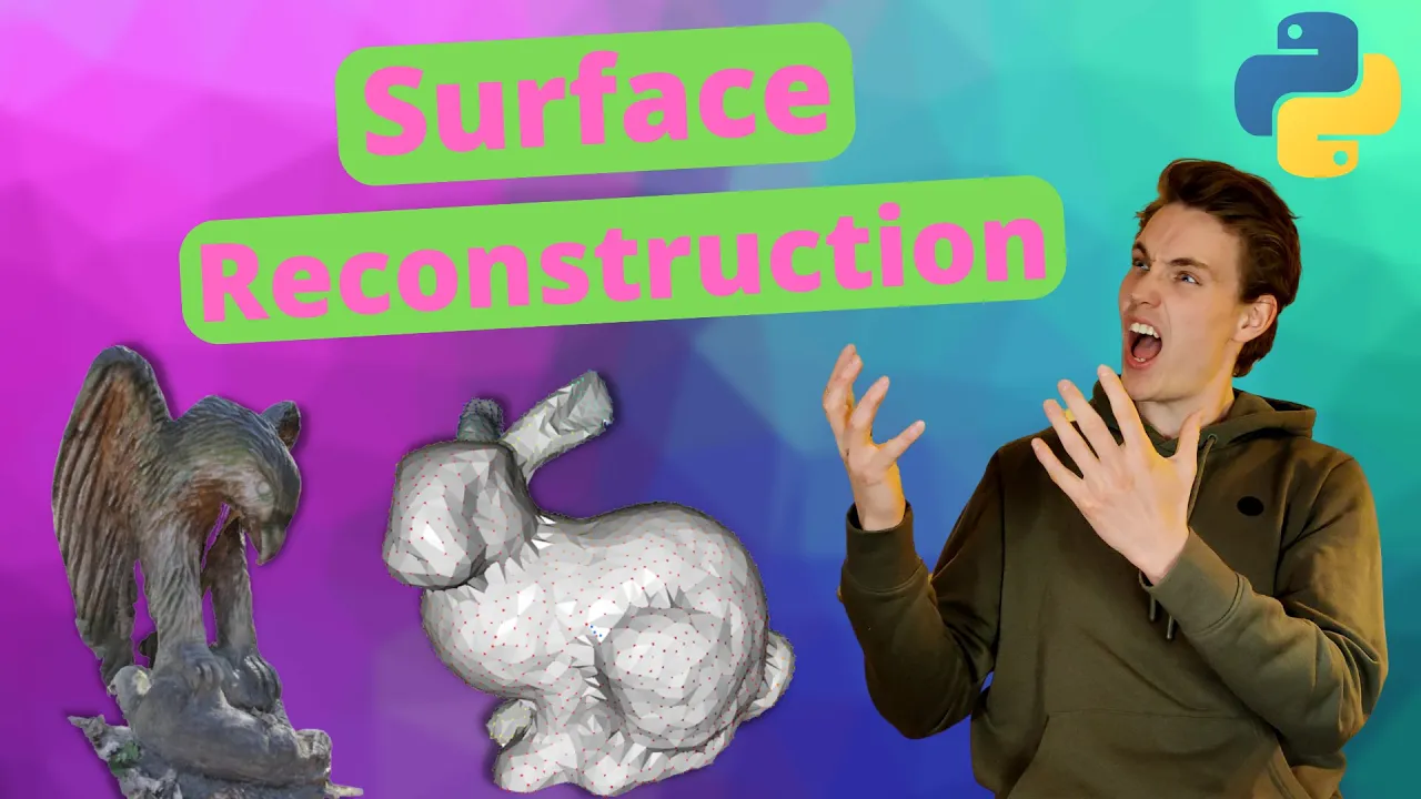
From Point Clouds to Surfaces: A Tutorial on Surface Reconstruction with Open3D and Python
23.8K
Surface reconstruction algorithms convert unstructured point clouds into triangle meshes by estimating surface geometry; Open3D implements three main methods: Alpha Shapes (generalized convex hull using an ice cream-chocolate analogy where points define boundaries), Ball Pivoting (dropping virtual balls to detect planar surfaces), and Poisson Surface Reconstruction (solving optimization problems with differential equations for smooth surfaces). The Poisson method is particularly effective as it can interpolate between points and extrapolate into areas of low point density, though it requires tuning parameters like octree depth and may benefit from intensity thresholding to remove unreliable regions.
Click to watch →
Deep Dive
Integrating 3D point cloud data into deep learning pipelines for object detection, segmentation, or classification (e.g., PointNet).
![[3D Point Cloud Data Processing] Capter 10. Overview of Deep Learning on Point-cloud](https://i.ytimg.com/vi/EPdlJ7WndMU/maxresdefault.jpg)
[3D Point Cloud Data Processing] Capter 10. Overview of Deep Learning on Point-cloud
1.4K
Point cloud deep learning enables five major application domains: (1) Classification - identifying object categories using ModelNet40 dataset, (2) Segmentation - assigning semantic labels to points including part segmentation (ShapeNet), indoor segmentation (ScanNet, S3DIS), and outdoor segmentation (KITTI, Waymo), (3) Object Detection - localizing multiple objects with 3D bounding boxes, (4) Registration - aligning point clouds using KITTI Odometry or 3DMatch datasets, and (5) 3D Shape Generation/Deformation - creating or transforming 3D meshes from sparse inputs.
Click to watch →

3D Computer Vision | 3D Point Cloud Processing
7.1K
This lecture introduces 3D point cloud processing, covering explicit representations (point clouds, meshes) versus implicit representations (occupancy grids, signed distance fields, neural radiance fields), followed by deep learning approaches including PointNet (which solves permutation invariance by processing each point independently through MLPs then applying max pooling) and PointNet++ (which adds hierarchical clustering via farthest point sampling and k-nearest neighbor grouping). The lecture covers six key tasks: place recognition (using PointNetVLAD with triplet loss for localization), key point detection/descriptor learning (using weakly-supervised approaches), 3D object detection (VoteNet with voting and clustering), semantic segmentation (weakly-supervised methods with smoothness constraints), point cloud registration (RPM-Net with Sinkhorn layers), and image-to-point cloud registration (combining deep learning classification with optimization).
Click to watch →
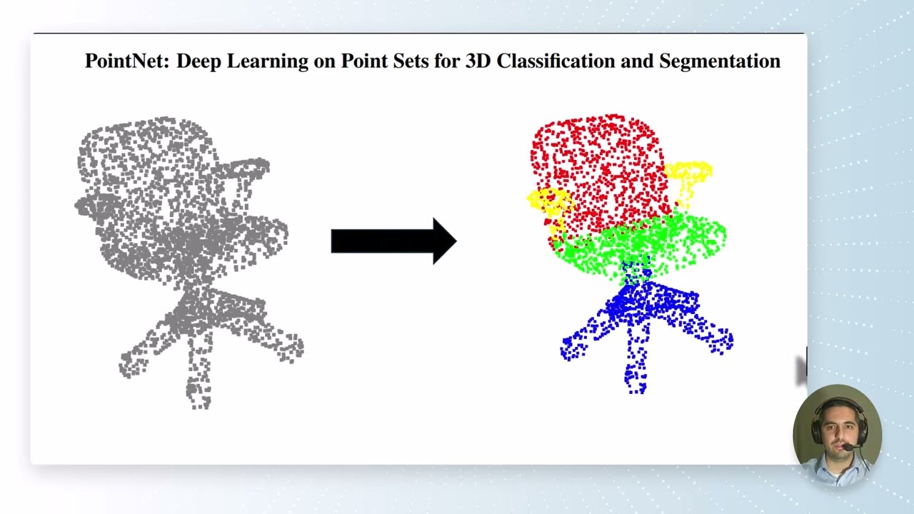
08 - 3D Point Cloud Segmentation with PointNet & OpenVINO| Deep Learning Tutorial
197
PointNet is a deep learning architecture for 3D point cloud segmentation that uses T-Net transformation networks for rotation invariance and max pooling for order invariance, enabling classification of individual points into semantic categories such as chair parts (seat, legs, back, arms) through a unified processing pipeline that transforms raw point cloud data into class-probability outputs.
Click to watch →
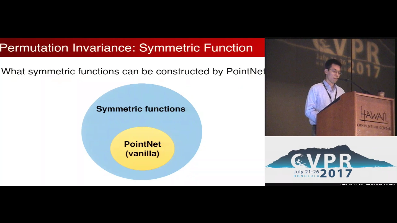
PointNet: Deep Learning on Point Sets for 3D Classification and Segmentation
69.2K
PointNet is a novel neural network architecture designed to directly process point cloud data by leveraging permutation invariance through symmetric functions, enabling unified solutions for 3D object classification, part segmentation, and scene semantic parsing while demonstrating robustness to data corruption and missing points.
Click to watch →
Open3D: A Modern Open-Source Library for 3D Data Processing
71.3K
Open3D is a modern, efficient, and easy-to-use open-source library for 3D data processing that implements fundamental data structures (point cloud, triangle mesh, voxel grid, octree) and algorithms (odometry, registration, TSDF volume integration) for applications in visualization, machine learning, and robotics; the library supports Python and C++ APIs, is cross-platform, and enables applications such as LIDAR semantic segmentation with PointNet++, 3D scene reconstruction with Intel RealSense cameras, and color map optimization, with future developments focusing on deep learning integration and GPU acceleration for real-time performance improvements.
Click to watch →
Point Cloud Creation
Laparoscopic Application
Point Cloud Creation
0:00- 1
Generates 3D point cloud from depth and RGB images using Open3D.
- 2
Converts images, sets camera intrinsics, and creates RGBD data.
- 3
Displays point cloud with adjustable view control for inspection.
Volumetric TSDF Fusion and Implicit Representations over Raw Point Clouds
While converting depth maps to raw point clouds using Python and Open3D is a standard geometric approach, it has significant limitations. Raw point clouds are discrete, unstructured, and highly sensitive to sensor noise and occlusions, making them inefficient for downstream tasks like rendering, physics simulation, or precise 3D reconstruction. A major alternative perspective advocates for volumetric integration methods, such as Truncated Signed Distance Field (TSDF) fusion, or modern implicit representations like Neural Radiance Fields (NeRFs) and 3D Gaussian Splatting. Instead of generating isolated 3D points, these methods fuse depth data into a continuous volumetric grid or neural field. This mathematical formulation naturally filters out sensor noise, resolves overlapping geometries, and directly generates closed, watertight meshes. Furthermore, for real-time applications like robotics, Python-based CPU processing introduces performance bottlenecks, leading industry practitioners to favor GPU-accelerated frameworks (e.g., PyTorch3D) or highly optimized C++ libraries (such as PCL) over standard Open3D Python implementations.
Basic Python programming, including familiarity with scientific computing libraries like NumPy.
Fundamentals of computer vision, specifically the pinhole camera model and lens distortion.
Understanding of camera intrinsic parameters (focal length, principal point) and coordinate systems.
The concept of depth images/maps and how they store spatial distance information per pixel.
Point cloud preprocessing operations, such as voxel downsampling, outlier removal, and normal estimation.
Point cloud registration techniques (e.g., Iterative Closest Point - ICP) to align and merge multiple 3D scans.
3D surface reconstruction methods (e.g., Poisson or Ball Pivoting algorithms) to convert point clouds into solid 3D meshes.
Integrating 3D point cloud data into deep learning pipelines for object detection, segmentation, or classification (e.g., PointNet).
389 views6likes3:13@pycp5998Original Release: 2024-08-18
hi welcome to another video in this video we are going to create Point cloud from depth image using open 3 and we also create Point Cloud for laparoscopic images let's start in my previous video I created depth map of an image using depth anything it will create RGB and gray dep images in the same code I added one additional function generate Point Club FN with the input parameters row frame and du inside the function first we will flip the image then we convert that image BGR to RGB then that image is converted to a num array and finally using geometry.
image we create that num array into open 3D image we have to do the same for depth image using Create from color and depth function we create rgbd image for creating the rgbd image both the raow image and the DU must have the same resolution before we create the point Cloud we need to create the camera intrinsic parameter and here I'm using the default parameters to get the correct depth in the point Cloud we can calibrate our camera to get the correct intrinsic parameters and load that into this function then create the accurate Point Cloud to create the point Cloud we can use Point Cloud do create from rgbd image and we can give the parameters rgbd image comma camera intrinsic for displaying the point Cloud we can use draw geometry function when you run the code the point CL will be upside down click and drag the mouse to see the 3D Point clock when you set a view contrl C and copy the Json parameters paste into the test editor copy the values front look at up and zoom add those values into the code when you run the code the point Cloud will show you the same view previously you copyed you can see input image depth map and 3D Point Cloud now let's create the point Cloud for laparoscopic image and here I using gr SK depth map here you can see the point cloud of laparoscopic image here you can see the laparoscopic surgery image grayscale depth map and 3D Point Cloud image we can improve the 3D output by calibrating the camera thanks for watching see you in the next video
Up Next

99:34
3D Point Cloud Processing Course: From Noise Removal to Segmentation
@FlorentPoux
2.9K views•2025-11-11

87:26
Introduction to Secure Multiparty Computation with Yehuda Lindell
@fhe_org
7.7K views•2021-02-04

4:55
HTTP Requests Explained: GET, POST, PUT, DELETE
@codecademy
103.1K views•2021-10-07

19:25
Enigma Machine Mechanics: WWII Encryption Explained
@JaredOwen
13.2M views•2021-12-11
Related Study Plans & Knowledge Roadmaps
Structured learning paths in Computer Science
computer-science
Container Runtimes: Namespaces, Cgroups & Go
01Linux Systems & Go Programming Foundations
02The Core of Isolation: Chroot and Filesystems
03Linux Namespaces: Process Isolation
+ 3 more learning modules
32h6 modules
Explore Roadmap
computer-science
Building a CHIP-8 Emulator: Rust & CPU Basics
01Computer Architecture Foundations (Bits & Bytes)
02Rust Programming for Systems Development
03CHIP-8 Virtual Hardware Specifications
+ 2 more learning modules
32h5 modules
Explore Roadmap
computer-science
Building BitTorrent: Go, P2P & Concurrency
01Go Fundamentals & Concurrency
02Networking Foundations & P2P Architecture
03Bencode Parsing & Torrent Metadata
+ 3 more learning modules
26h6 modules
Explore Roadmap
computer-science
Actor Models (C++ Concurrency & Lock-Free)
01C++ Multi-Threading Foundations
02Thread Pools and Task Scheduling
03Atomics and Lock-Free Queue Design
+ 3 more learning modules
45h6 modules
Explore Roadmap