














![doc. P. Hušek: Lineární systémy (B3M35LSY1) – 10a [28. 11. 2023, ZS 23/24]](https://i.ytimg.com/vi/g1szIlq8Mkw/maxresdefault.jpg)



![Control [1] Section (7) : State Space Forms Part2](https://i.ytimg.com/vi/gYQVEwhGJCQ/maxresdefault.jpg)

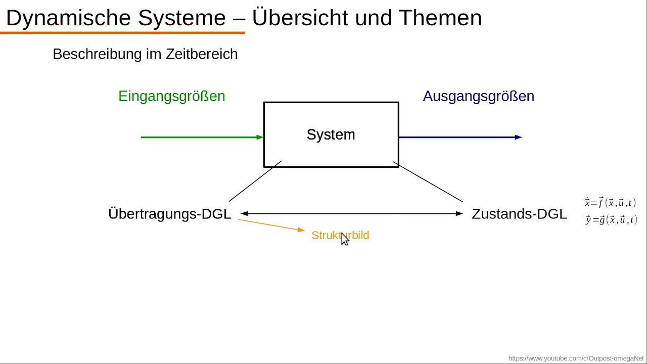
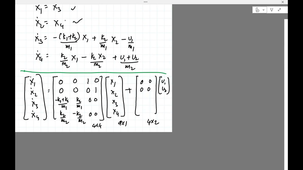
State space representation transforms high-order differential equations into a system of first-order differential equations in the form X_dot = AX + BU (state equation) and Y = CX + DU (output equation), enabling efficient analysis using linear algebra tools for stability assessment, control system design for multi-input multi-output (MIMO) systems, and numerical simulation; the process involves identifying inputs, outputs, and defining states, with the total system order being conserved in the transformation.
State Space Representation of Dynamic Systems: An Introduction
Added:Fundamentals of Ordinary Differential Equations (ODEs), particularly high-order linear differential equations used to model physical systems.
Basic Linear Algebra concepts, including matrices, vectors, matrix multiplication, and systems of linear equations.
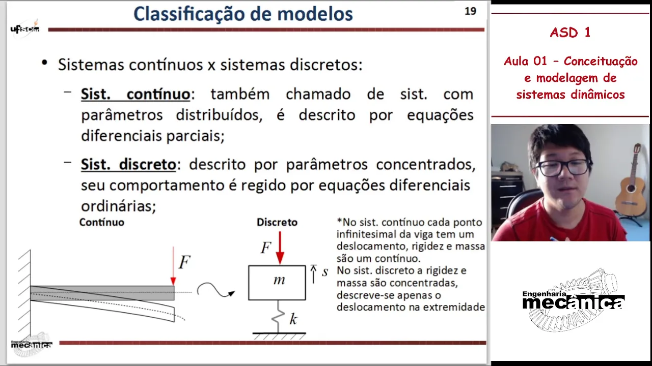
Core concepts of dynamic systems, such as inputs, outputs, and system variables in physical domains (e.g., mechanical or electrical).
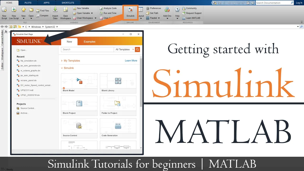
Introductory familiarity with MATLAB and the Simulink graphical simulation environment.
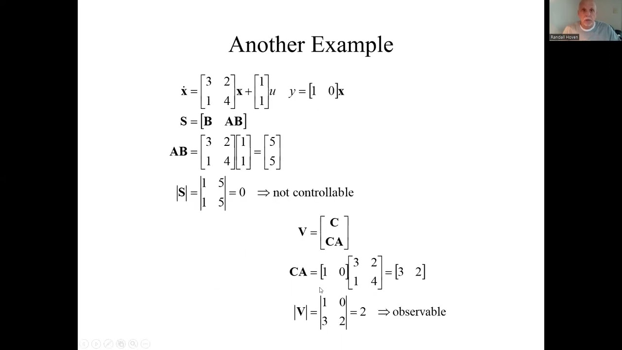
Analyzing system properties, specifically Controllability and Observability, using the state-space matrices.
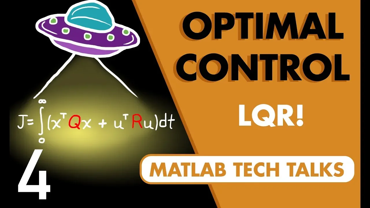
Designing state-feedback control systems using techniques like Pole Placement and Linear Quadratic Regulator (LQR).
Constructing State Observers (such as Luenberger Observers) to estimate internal states that cannot be directly measured.
Converting between Transfer Functions and State-Space Canonical Forms (e.g., controllable, observable, and diagonal forms).
74.8K views420likes21:56Original Release: 2014-01-08
hi this is Gordon Parker from Michigan Tech and today we're going to be doing an introduction to State space representation of dynamic systems okay so what we're going to do in this short video is look at two questions why and what we're also going to do just a little bit of simulation really that's just to see a practical application of this state space representation business okay um so why well actually why don't we start with what first so let's do the what part first um let's say that you have a denamic system that has or is described by a couple differential equations so so here's one in Theta it actually has Theta triple dot a Theta double dot a Theta and let's say it has an input to one some kind of a torque and then we have another dynamic system that is described by these equations and it has an input to two so we have um a little bit of coupling between these two Dynamic systems uh primarily in this equation it has the Theta uh variable in it so we have this thing and and often times we want to solve it or come up with a uh simulation of it and in state variable form what we do is is we transform this set of two differential equations this one being third order and this one being second order right it has three derivatives up here so it's third order this one's second order because it has two derivatives we're going to transform those into a system of first order differen equations that has this form X do = ax + bu U and I'm using a single underbar for a vector and a double underbar to denote a matrix we call this equation the state equation and in state variable form we also generate another equation that on the right hand side really has the identical form of the state equation except we use matrices c and d and this one is called the output equation so the act of converting this differential equation or set of differential equations into State variable form is really just the act of determining four things the matrices a b c and D of course to get there there are a few extra steps we have to do things like um Define what the inputs are or identify what they are in this particular example the inputs were t one and to2 normally this is dictated by the the physical structure of the system that you're working with we also have to identify or Define what the outputs are right and the inputs by the way we typically denote those as U so you know here's where the inputs uh enter into the the state equation and the output equation the outputs are typically denoted as Y and we haven't really said what they are in this case maybe a reasonable output would be a Theta uh maybe a Theta Dot and perhaps an alpha there's three outputs I don't know again it depends on what it is you're doing with that analysis and we typically denote those go with Y the biggest thing that you have to do is you have to come up with a definition of the states and in these equations the states are denoted as X and I'm not going to say what they are in this particular example because we haven't defined them yet we'll actually do that um in a short example in just a minute and then in a more detailed example in another video okay so again what it is is converting it's a representation of a dynamic system in first order form first order because I have a single dot there and um it is defined in terms of inputs outputs and these things called States so now let's look at why we would do such a thing and just as a a reminder I'm just going to rewrite this and I would highly recommend that you just get in the habit of writing this out whenever you're dealing with um State space analysis of design okay um again first order set of differential equations um why do we do this well there's really an analysis Advantage right in the previous Slide the previous page we had two sort of high order differential equations one was third order and one was second order when we get it into this form what we actually end up with and just as a reminder we were third order in Theta we were second order in Alpha and what we'll end up with here if we convert this into State space form is an x dot that has that's a 5x1 Vector okay so we end up with five of these first order differential equations so there's a certain conservation of of order here um you know third order plus second orders there's five we're not going to increase or decrease that order by going to State space form however it gives us a nice clean representation an A and A C and A D Matrix and what that allows us to do is use all kinds of results from linear algebra to Analyze This system so for instance we can analyze its stability incredibly easily um just by looking at the a matrix and Performing some operations on it um we can also get information about the characteristic response of the system and uh what I mean by that is or I should say an example of that is things like um determining its igen values or if you are familiar with the lass domain representation of a dynamic system um finding the poles of this dynamic system simply by looking and doing some operations on it in this uh Matrix form um we can also do control system design very effectively now couple words on that so if if you've had a course in automatic controls typically what you did is you looked at single input single output systems so call those ciso so it's single input single in single out okay um now in the previous in the example on the previous page I had two inputs a tow one and a tow two we had three outputs a Theta a Theta Dot and an alpha it was definitely not single input single output we call those types of systems multiple input multiple output now if you had that course in automatic controls or you've done some um design of single input single output Control Systems it's not too bad to do um but extending that to multiple input multiple output can be very tedious um using you know typical methods block diagrams and that sort of thing but when we put it in the state space form again we can utilize all these wonderful uh uh tools from linear algebra to do the mimo multiple input multiple output control system design and then finally one more thing is simulation or um you know numerical solution now on the previous page we were third order in Theta second order and Alpha a couple differential equations and couple um solving those is for linear systems is possible um perhaps depending on you know what we're doing with it um uh but numerical solution really requires you to put it into this first order form this state space form whether the system of equations is linear or nonlinear so it gives us a great way to um uh a great leg up on doing simulations so that being said let's just do a little example of that um let's see what I'll do is do a just a incredibly simple um system we'll just take this one and maybe I'll title this as simulation example what El do is I'm going to take a a second order differential equation in Theta and there's an input five tow okay beautiful second order differential equation in Theta the input is too and um if you do have a background in in uh the laass domain you know you could come up with a transfer function of this so Capital Theta of s over capital to of s is equal to 5 over S2 + 3s + 5 or 13 I'm sorry and you know you could analyze the heck out of this thing you can look at it poles etc etc uh you could put it into a tool like simulink as a transfer function give it a some type of an input a step input and get a response or we could put it into State variable form and if we I'll just run through how we would do that in this uh simple example we'll have two states and I'm going to define those two states as X1 and X2 and X1 will be Theta and X2 is Theta dot now I'm just defining those it turns out there's an infinite number of ways to represent this system in state variable form by defining the states this way I've sort of vectored myself in a unique representation um but that's one of the disturbing features for people just learning State variable or state space representation is that there's no one correct answer there's an infinite number of them um now remember in state variable form remember I I did say it's handy to write this down a bunch of times what we're really looking for is x dot as a function of X and the input U now in our case our input is is TOA I shouldn't have done that that's not a vector it's just a thing that I wanted to point to and our states are defined over here X1 and X2 but what I need is x dot so I'm just going to say X1 dot X2 dot equals equals X1 dot is equal to Theta Dot and if I want to put it in terms of X that's X2 and X2 dot is Theta Dot and that is nowhere to be seen in our state variable definition however I can get it straight from this equation specifically it's -3 Theta dot -3 Theta and plus 5 and instead of to I'll just call it U and so that's -3 Theta dot is X2 and Theta is X1 and again we have this input basically done I can write my State equation um the way I like to do that is I just kind of hog out some space on the page for my a matrix I hog out some space for my B turns out it's just a vector and then I start filling in the blanks so to speak so from that first row I get it from this X1 dot equation and all that's in it is an X2 and there's no input for the second equation it's a -3 a -3 and a five so there's my state variable my state equation again don't worry too much about the details of how I did this we'll have that in gory detail in another video really I just want to get to a state varable form and then simulate the stinker um let's say that my output for this example is Theta so I'm going to say my y is equal to again I hog out some space for my C Matrix because remember Y is equal to CX plus duu so I hog out some space for my C and I hog out just a wee bit of space for my D since my output is Theta Theta is really just X1 so I pick up a one there a zero there and a zero there I'm I'm done I have my a my B my C and my D Matrix and so now it's just a matter of putting it into some sort of simulation tool so let's go ahead and do that so you'll see some things kind of blinking around a bit on the screen as I switch over [Music] to um actually I don't even need that that I can just go straight to simulink and I'm just going to say file new model and over here in the pallet of different blocks I'm going to go over to continuous and you notice that um there is a state space block right here so I'll just drag and drop that in with a left click might be a little bit hard to see in in uh uh with the resolution here but um we'll just keep going forward um so now I just put in my a b c and d Matrix so let's see my a is 01 semicon -3 space3 and my B Matrix is what was my B Matrix 0 five whoops um 0 five and my C Matrix was 1 Z and my D Matrix was just a very lonely zero now initial conditions I have two states and so I need to specify two initial conditions uh I'll just go z0 and I'm done and let's force feed this one some sort of an input I go to sources how about a step input so I'm going to put a step in tow and if I double click on step uh the step is going to start at time equal one has an initial value of zero and a final value of one it's fine and let's put it to an output or a sync in the mat lab terminology now let's use a scope and I can even label this as um X my state Vector X so it's actually going to have two uh traces in it now we'll go up here to my um configuration of the simulation and I'll just change a couple things start time is zero start stop time is 10 um I'll use a fixed solver od3 is fine and I'll use 100 Herz 01 and we hit the green button it dings double click this and whoops oh I'm sorry I said that there would be two traces actually there's not because we only had one uh output it was Theta and look at that your basic second order response is overshoot sing time all these interesting time domain characteristics it starts at 1 second and away it goes if I wanted to see both States I can easily do that by going into the C Matrix and changing it to um one Zer that will pick up the first state 01 will pick up the second state and then over here I'll need to to add another um zero to my D Matrix so with that simple change I can rerun it and now I have this my yellow is Theta and my pink is Theta dot or the speed so as we see Theta going to a constant value of course the speed is going to zero that would be a lot harder to get with a transfer function with a transfer function we could have gotten the yellow one no problem but the pink one we would have had to jump through an extra hoop or two um and just to see that we can go over here to continuous and grab a transfer function and I'm going to put into it the transfer function that I wrote down at the beginning of this example I think it was 5 over 1 3 and 13 and I'm going to drag this same input into it go back here I'm going to grab um just another scope I guess and I can just right click this and drag it to make a copy and here I'm going to call this one X but from a transfer function run it bling Bing whatever and there's our output from the transfer function I'm going to try to make it about the same size as this one uh actually that's kind of cheesy but um you get the idea a much better way to to convince ourselves whoops that the two yellow traces are the same because they don't look at it here because the scales are all different is to do something really simple here I'm just going to take a math operation and grab an add block and make one of these so I double clicked on it but I'll make one of these a minus and I'll grab this one let me stretch this out a wee bit just clean stuff off Tad this one there one more scope guess what I have now I have the error between my state space representation of that dynamic system and a transfer function representation run that and oh of course I did pick up both the yellow and the pink States so if I wanted to go back to the um the single output case that that I had down on the paper or I should say on the um slide would look like that oops what have I done wrong ah so this should be one zero there we go and run that look at my error it's beautiful it's zero so this is just to illustrate that that transfer function representation and the state space representation are the same thing we got a little bit of numerical um Jitter in there a little bit of noise but that's just an artifact of of how those two different how those two systems were solved slightly differently numerically so that's it quick intro to uh State space we covered uh what they are right you take a bunch of differential equations of potentially high order and represent them as first order differential equations making sure that you identify what the inputs are what the outputs are and Define some states we looked at why we do this um it has to do with efficient analysis using linear algebra tools efficient control design for mimo systems multiple input multiple output and then finally we looked at one of the the big aspects one of the more important aspects of why and that is easy numerical simulation thanks
Up Next
13:03
LQR Control for the Inverted Pendulum on a Cart: Full-State Design
@Eigensteve
243.5K views•2017-01-29

30:32
Ultrasonic Transducers: Resonant Frequency Measurement and Horn Design
@imajeenyus42
229.9K views•2017-02-22

54:16
Polymer Environmental Degradation: Mechanisms & Stabilization
@iit
1.8K views•2012-07-10

33:39
How a Student's Question Saved a NYC Skyscraper from Collapse
@veritasium
22.8M views•2025-04-26
Related Study Plans & Knowledge Roadmaps
Structured learning paths in Engineering
engineering
Building Acoustic Levitators: Physics & Arduino
01The Physics of Sound and Standing Waves
02Piezoelectric Transducers and H-Bridge Drivers
03Arduino Programming: Generating 40 kHz Signals
+ 2 more learning modules
14h5 modules
Explore Roadmap
engineering
Building Peltier Cloud Chambers: Particle Tracks
01Cosmic Rays & Cloud Chamber Physics
02Thermoelectric Cooling (TEC) Fundamentals
03Custom Liquid-Cooling Loop Design
+ 2 more learning modules
18h5 modules
Explore Roadmap
engineering
Yagi-Uda Antennas: Modeling, Build & VNA Test
01Introduction to RF and Antenna Fundamentals
02Yagi-Uda Antenna Design Principles
03Antenna Modeling and Simulation in 4NEC2
+ 2 more learning modules
18h5 modules
Explore Roadmap
engineering
ECG Monitor Design: Op-Amps, Filters & Noise
01Electronics & Breadboard Basics
02Op-Amps and Instrumentation Amplifiers
03Bioelectricity and ECG Fundamentals
+ 2 more learning modules
18h5 modules
Explore Roadmap