







![ปูพื้นฐานการใช้ Python ร่วมกับ NumPy | สำหรับงาน Data Science [FULL COURSE]](https://i.ytimg.com/vi/MDA8SbfdLKA/hqdefault.jpg)




![Me Salva! [AO VIVO] Revisão de Física (Cinemática) para o Ensino Superior](https://i.ytimg.com/vi_webp/bdj0wk3t4Lg/maxresdefault.webp)
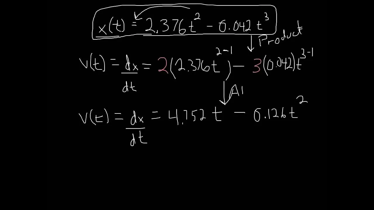



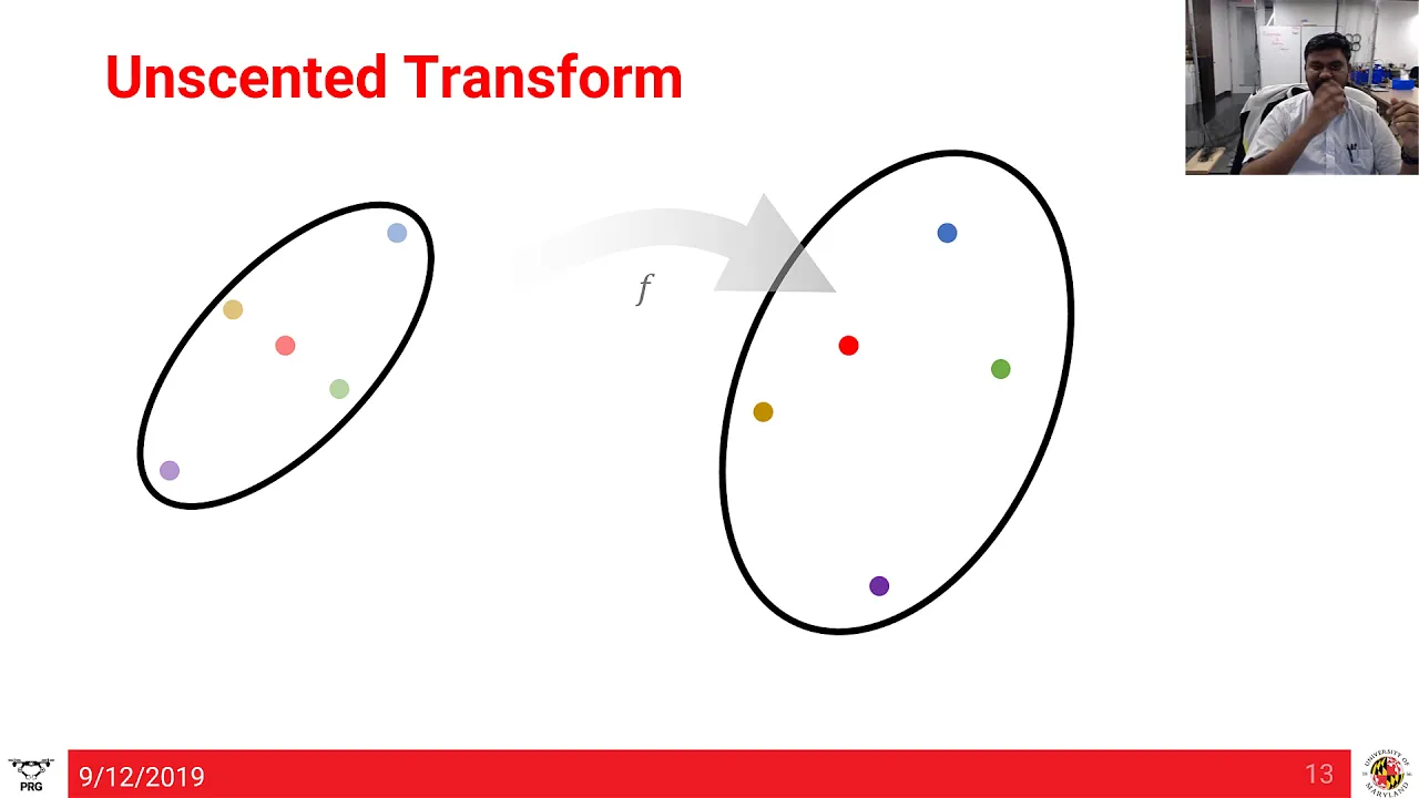






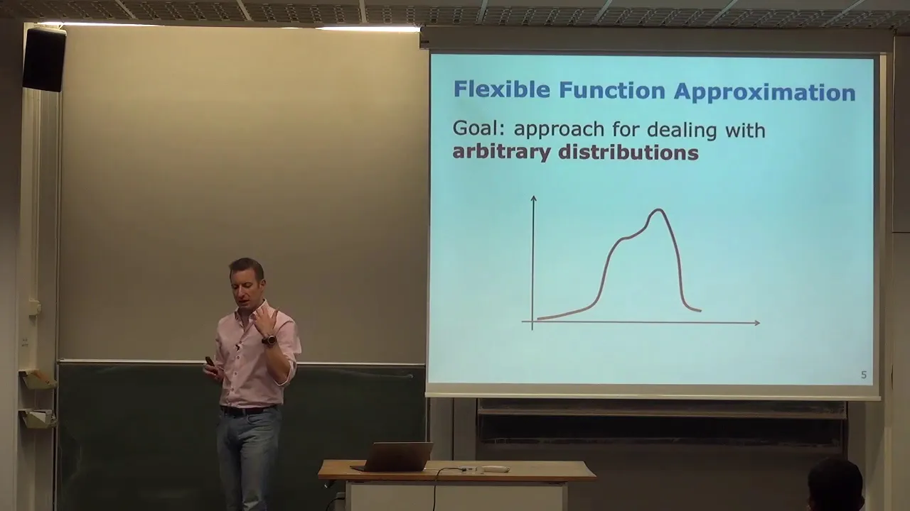

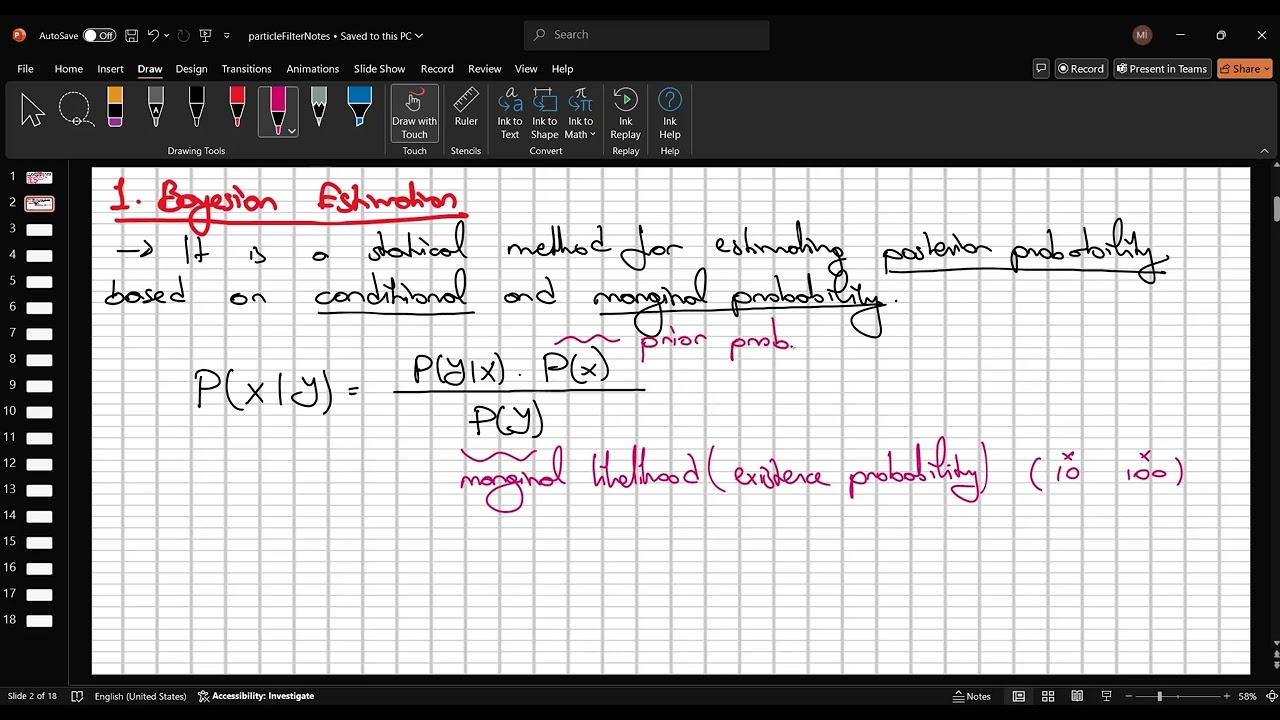
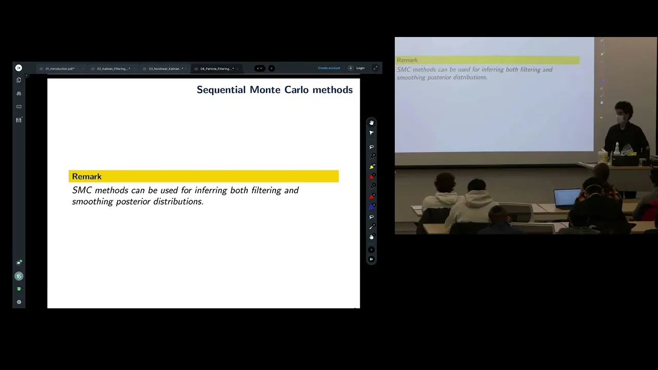
The Kalman filter is an algorithm that combines predictions from a motion model with sensor measurements to estimate the true state of a system, where the filter alternates between a prediction step (forecasting the state based on control inputs and motion model) and an update step (refining the estimate using sensor data), with the key insight being that the true state lies at the intersection of the motion prediction and sensor measurement, and the filter's gain determines how much weight to give to each source of information.
Understanding Kalman Filters: Intuitive Tutorial for Beginners
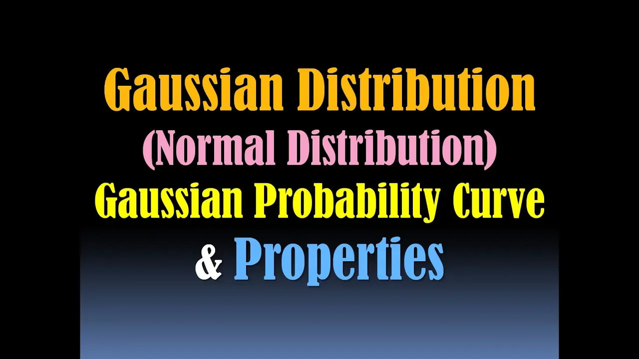
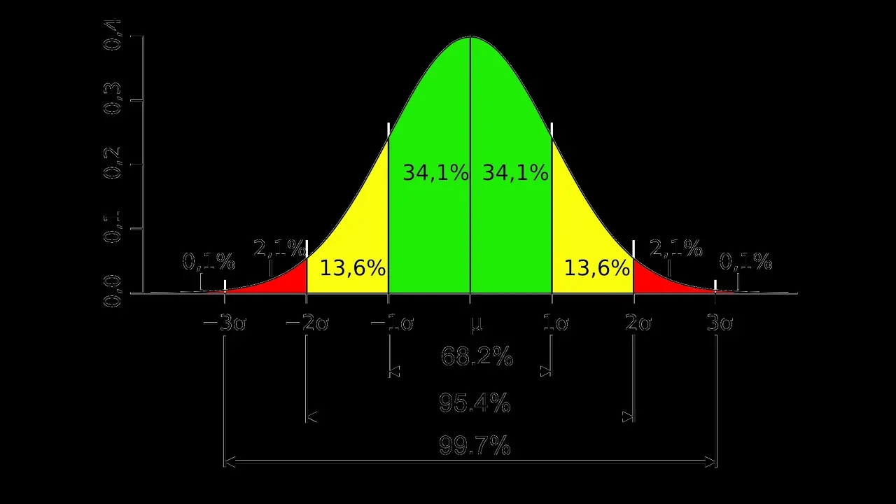
Added:Basic probability concepts, specifically Gaussian (normal) distributions, mean, variance, and covariance.
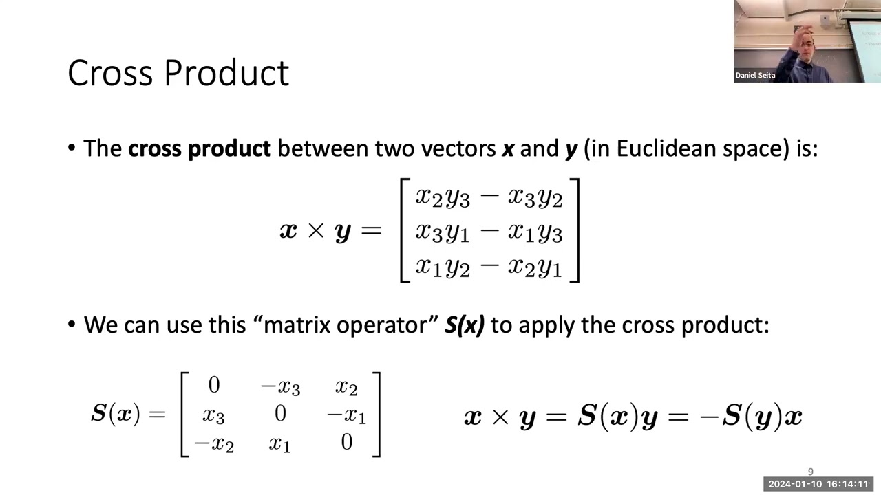
Fundamentals of linear algebra, including vector and matrix operations such as multiplication, transposition, and inversion.
Basic Python programming proficiency, particularly familiarity with the NumPy library for array and matrix manipulation.
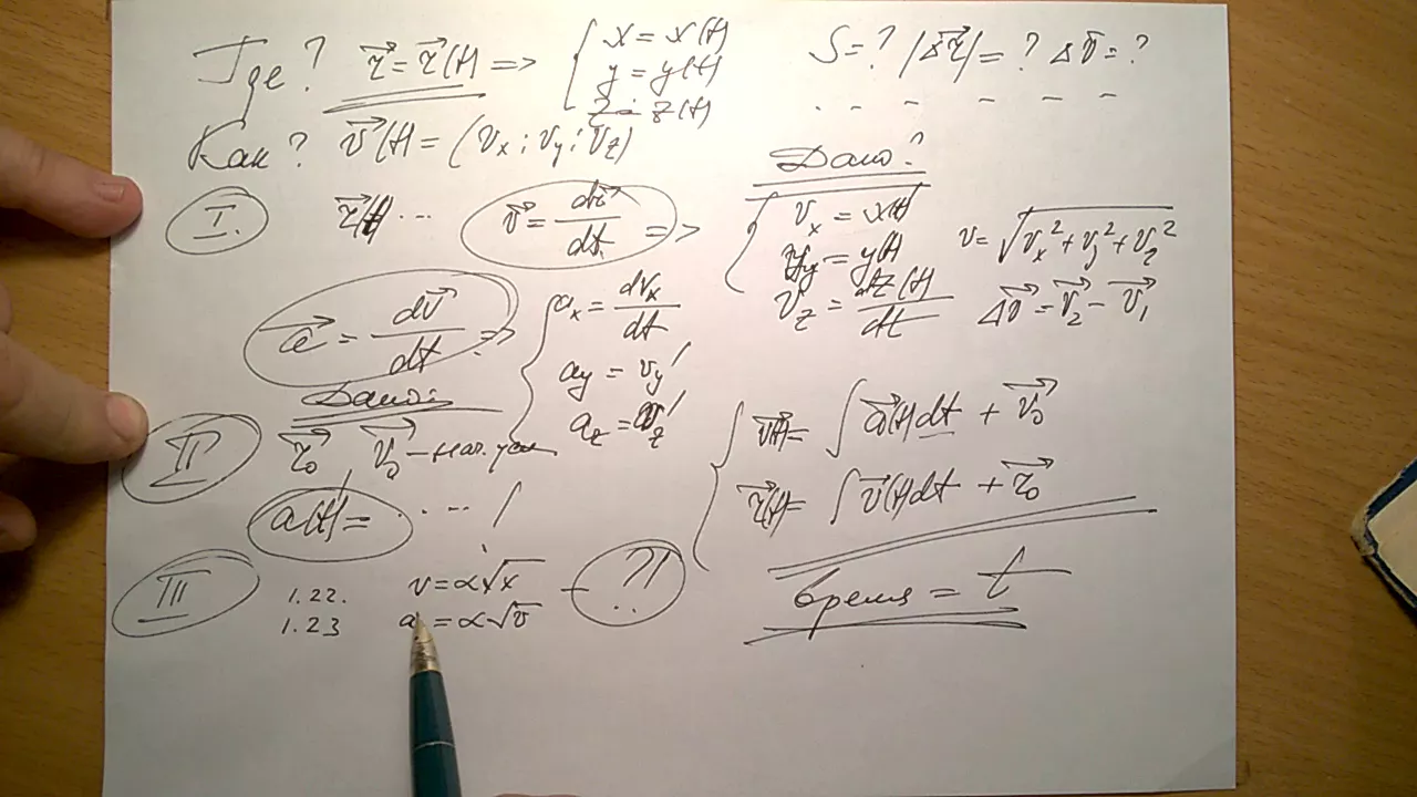
Elementary physics or kinematics concepts, such as the state representation of position, velocity, and acceleration.
The formal mathematical derivation of the Kalman Filter equations using Bayesian inference and least-squares estimation.
Extended Kalman Filters (EKF) and Unscented Kalman Filters (UKF) for handling non-linear system dynamics.
Practical sensor fusion applications, such as combining accelerometer, gyroscope, and GPS data for autonomous vehicle localization.
Particle Filters (Sequential Monte Carlo methods) to address non-Gaussian noise and highly non-linear state estimation problems.
14.7K views347likes8:09Original Release: 2021-01-10
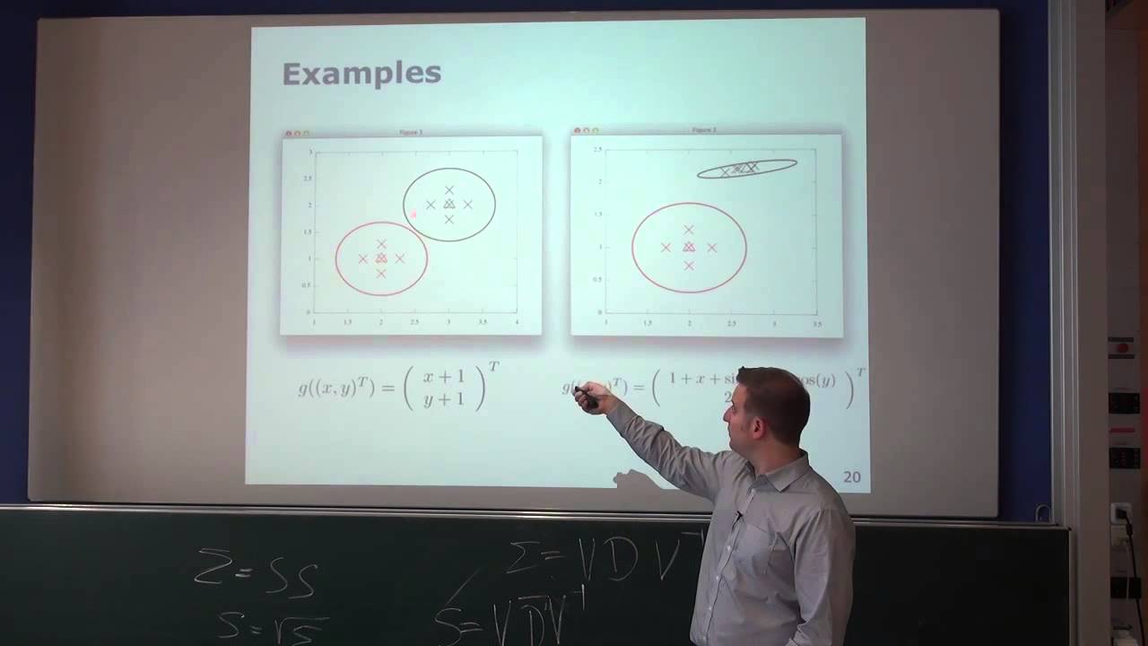
today we'll talk about probably one of the most well-known estimation algorithms called the common filter when i first learned a few years ago i wasn't able to grasp the intuition on what common filter is doing and how to actually implement it to me and at least to some others that i know was mainly because we started by going through all the complicated derivations of the common filter equations and by the end of it our brains were already exhausted and we didn't even remember anymore why we dragged it in the first place so today i want to try something different i'm gonna split the discussion of the common filter into three parts the first part is about what common filter is and how to use it second is on how to actually code it and for those interested the third part is about the derivation of the common filter equations in this video we'll only focus on the first part to understand this also assume that we already know some basic knowledge about multivariate gaussian and state space system so instead of deriving all the equations i'm just going to give you all the equations that we need to actually implement the common filter don't get me wrong i think understanding how the common filter equations are derived is important and can give us additional insights on how kalman filter actually works but let's not do that here so we can focus on the intuition let's get started a state describes the condition for a watt at a specific time for example a location of a robot on a 2d plane can be considered as a state state estimation is the problem of estimating the state of a robot from noisy data in the real world we may already know the motion model of our robot that allows us to track how the state of robot changes over time given its initial state and applied control signals at each time step unfortunately the motion model is never perfect this can be because of imperfect parts of the robots and many other reasons so relying only on the motion model to do the estimation can only give us noisy state estimates okay but robots typically have various sensors on it can we just take the measurement from the sensors to get the state of our robot well sensors are also not perfect and typically are noisy but now seems like we have two different ways to get some sort of state estimates each with known uncertainty so can we combine the prediction from our motion model with the sensor measurements to get better state estimate and this is where the common filter can help us if we have additional information about the state of our robot as long as they are somewhat informative we can combine this information using common filter to get a better state estimate the intuition is that the molecule state is probably the state that falls between the intersection of the motion model and the sensor measurement now the question is how do we concretely combine this information before we talk about questions let's first talk about the assumptions used in common filter first we assume that robot has a linear motion model with gaussian noise so we can write the equation that explains how the state changes as we apply a control signal in this form second we also assume the robot to have a linear measurement model with gaussian noise finally we assume caution prior for the initial state of the robot of course these assumptions sometimes are not realistic but they allow us to derive the equation for the common filter it turns out that even with these assumptions common filter is still powerful technique that we can often rely on in the real world okay so now we're getting into the common filter equations there are two main steps that we need to perform we call these prediction and update steps the goal prediction step is to predict the state of the robot based on the motion model after we apply a control signal and this is the equation we need for the prediction step since the model is cautioned the prediction of the belief state is also cautioned and since gaussian is paralyzed by the mean and covariance we want to compute the new mean and the new covariance after applying the control signal here the mean signifies our belief of where the robot is after we apply the control signal while the covariance represents our uncertainty after we do the prediction step we shouldn't have received a measurement zt from our sensor the goal of the update step is to update the belief that we just computed from the prediction step by considering the measurement that we just received from our sensor the uncertainty in the belief state should then decrease as a result of the update step now this is where i'm going to start giving into common filter equations without actually deriving them these are the equations that we need to perform the update step the first equation is to compute the residual or the difference between the sensor measurement and our latest prediction the second equation is to compute what is known as the common gain common gain can be thought of as some sort of ratio and it determines whether we trust the measurement more or the prediction finally we compute our new belief state using the residual and the common gate and as we can see here if the common gain is high the new belief is largely affected by the sensor measurement again we're not going to go through the derivation that gives us all the equations for the update step but i hope this can still help us to at least understand how common filter can be used and what is actually needed to implement it now let's take a look at a concrete example to see how we can use these equations imagine a robot moving in a room without obstacles the robot is equipped with a sensor to measure its location in the room these sensors are not perfect however the manufacturer provides us with information that tells us how inaccurate the sensors are in addition we also know the motion model of the robot we are using this means that we know the a b q h and r matrices let's say that these are the matrices say the state of the robot is its x and y position in the room and the control inputs are the velocity in both x and y direction the initial belief of the robot is that the robot is located at 0 0 with sigma 0 as the uncertainty and the robot moves with constant control inputs the question is what is the state estimation after one time step if the measurement the robot gets after applying the control commands at t is 0.93 and 1.77 to enter this we just need to use all the given information to perform the prediction step followed by the update step first let's do the prediction step we literally just take the equation and plot all the available information to that equation and we'll get this as a new belief of where the robot is currently at after prediction step we take the measurement data and perform the update step again we just need to take all the information we need and plug that into the equations so first we compute the residual and then we compute the common gain and then we finally compute the new belief and this is our state estimation after one time step [Applause] let's do a quick recap so we have a robot in the room and we have an initial belief of where the robot is currently at this initial belief is represented as mu 0 and sigma 0.
the state of the robot is its x and y coordinates and the robot is moving with a constant velocity ut after we apply the control signal ut the robot moves and so does our belief to get the new belief we perform the predicts that this new belief represents where we think the robot is currently at based on the noisy motion model after we perform the predict step we assure the robot to have received our center measurements at t and once we have zt we perform the update step by first computing the residual the common gain and finally the updated belief as a result of the update step the uncertainty of the updated belief should decrease and this makes sense because we just used some new information from our sensors about the state of the robot to update our belief you see once we have the equations for the common filter it's not actually that hard to implement the common filter in terms of coding we just literally need to write two functions one for the prediction step and one for the update step so that's it for today's video in the next video we'll take a look at how to actually implement the common filter in python using only numpy see you next time
Up Next
70:36
Machine Learning for BCI: Challenges & Best Practices (Tutorial)
@bcisociety6038
2.5K views•2021-02-17

57:48
Secure Multiparty Computation (MPC): Foundations & Challenges
@SimonsInstitute
7.3K views•2015-05-28

13:03
Bypassing Tor Censorship: Bridges and Pluggable Transport Guide
@Coding_ForEveryone
397 views•2024-06-11

18:41
Neural Networks Explained: Math, Layers, and Learning Fundamentals
@3blue1brown
21.9M views•2017-10-05
Related Study Plans & Knowledge Roadmaps
Structured learning paths in Artificial Intelligence
artificial-intelligence
Aligning LLMs: DPO, TRL & Custom Datasets
01Foundations of Python & Machine Learning
02Transformers and Large Language Models (LLMs)
03Aligning LLMs: SFT and RLHF
+ 3 more learning modules
24h6 modules
Explore Roadmap
artificial-intelligence
Federated Learning: PyTorch, Flower & Privacy
01Python & Machine Learning Foundations
02Deep Learning Basics with PyTorch
03Introduction to Federated Learning
+ 2 more learning modules
35h5 modules
Explore Roadmap
artificial-intelligence
Securing LLMs: Guardrails AI & NeMo Gateway
01Introduction to LLMs, Python, and APIs
02Understanding LLM Vulnerabilities & Threats
03Defending LLMs with Guardrails AI
+ 2 more learning modules
15h5 modules
Explore Roadmap
artificial-intelligence
Building Recommenders: Two-Tower & Vector DBs
01Foundations of Python & Machine Learning Basics
02Introduction to Recommender Systems
03Deep Learning & Representation Learning
+ 3 more learning modules
75h6 modules
Explore Roadmap