
![Master matematika kursi (130-dars) [4637-...4670]-misollar](https://i.ytimg.com/vi/c04k5hzYpxA/sddefault.jpg)


![How Rotary Encoder Works and How To Use It with Arduino[with CODE] | Arduino Encoder code explained](https://i.ytimg.com/vi_webp/wNuuMXGxm3g/maxresdefault.webp)





![[물리를 이해하며 함께하는 수학, 무리함수] 라그랑주 역학과 뉴턴 역학, 최소강하곡선 문제](https://i.ytimg.com/vi/TfS9uq6e1i4/maxresdefault.jpg)



![[경희대 김동한] 2021-2 센서기반모바일로봇 (1-2)](https://i.ytimg.com/vi/AsAm0Pjw9LE/sddefault.jpg)




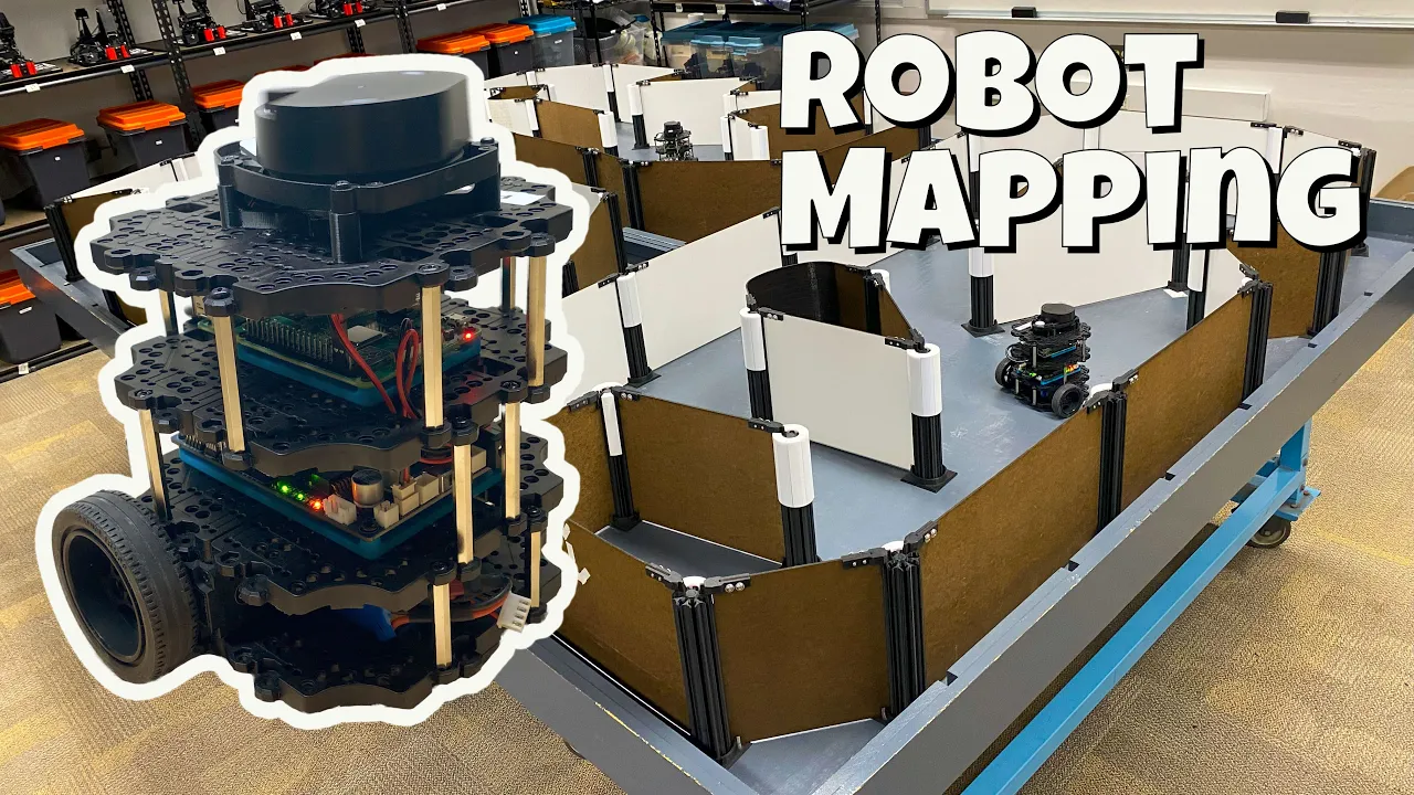

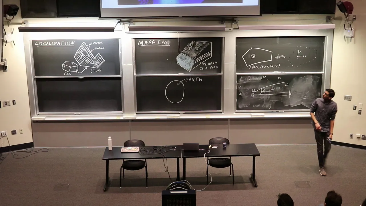


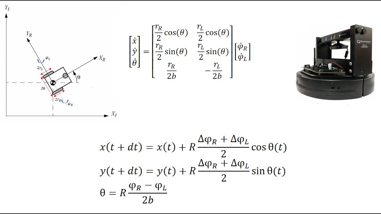
This video explains how differential drive robots use wheel encoders to compute odometry (position and orientation) through geometric modeling. The key formulas are: distance traveled by each wheel DL = ((SL - S_prev)/Q) × C, change in orientation Δθ = (DR - DL)/(2×RW), and change in position D = (DL + DR)/2. For velocity, linear velocity V = (VL + VR)/2 and angular velocity θ̇ = (R × (VR - VL))/(2×RW). The fundamental non-holonomic constraint for differential drive robots is Ẏ × cos(θ) - Ẋ × sin(θ) = 0, meaning robots cannot move sideways instantaneously—they must rotate and translate simultaneously.
Wheeled Robot Control: Differential Drive Odometry Tutorial
Added:Basic trigonometry and 2D coordinate transformations, including translation and rotation in a Cartesian plane.
The working principles of rotary wheel encoders and how they translate physical wheel rotations into digital ticks.
Fundamental concepts of linear and angular velocity, along with basic calculus for time-integration.
An introductory understanding of kinematics, specifically the difference between holonomic and non-holonomic constraints.
Analyzing and mathematically modeling cumulative odometry error propagation (drift) over time.
Implementing sensor fusion techniques (such as the Extended Kalman Filter) to combine wheel odometry with IMU and GPS sensor data.
Designing motion control algorithms (like PID controllers or Pure Pursuit) to guide the robot along a desired trajectory using odometry feedback.
Exploring simultaneous localization and mapping (SLAM) frameworks that rely on odometry as a primary motion model input.
53.2K views1.4Klikes42:15Original Release: 2019-09-11
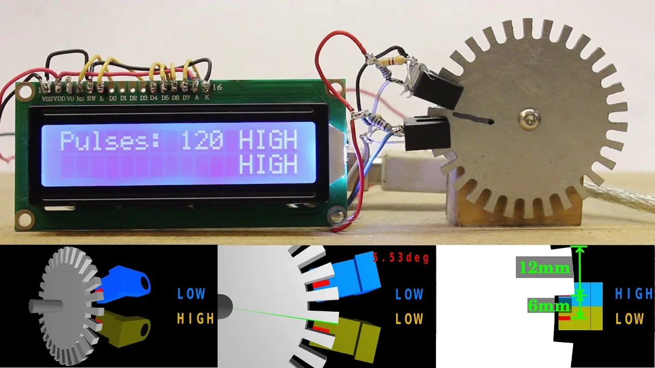
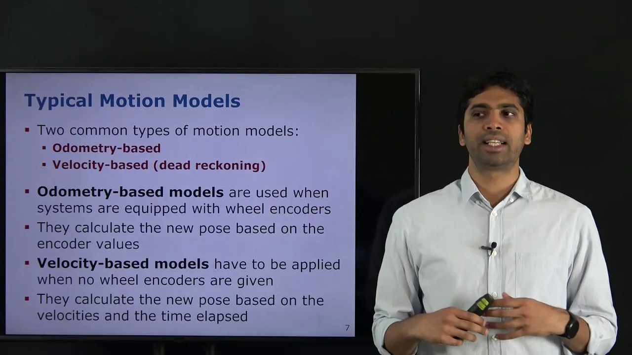
the first big topic that we're going to talk about in this class is wheeled robot control and we specify wheeled robots because there are just so many different types of robots I list a few of them here wheeled robots are you know kind of self-explanatory they're any robot that moves with wheels so self-driving cars would be a wheeled robots the the robot we looked at in class earlier was a wheeled robot there are other types called manipulators and those are kind of like the technical term for robot arms those are a whole class of robots in themselves their legs robots these are typically robots that are moving on the ground but not moving with wheels so think of like humanoids or you know you may have seen like cheetah robot videos over the last few years but then of course there are aerial robots and you know these are just any robots that fly and drones comprise the largest percentage of those kinds of robots but we're just gonna be focused on real robots for this class and they're even within wheeled robots there are quite a few different types here are just four common types on the far left we have differential Drive robots which is what the turtle bot 3 is it has two wheels moving independently of one another and shown here I have the base of the turtle bot 2 which also is a differential Drive robot car like robots are of course wheeled robots there are a couple others called skid steer in synchro we won't really work with any of those in this class and we won't even really mention them much I if you continue in a robotics industry you'll probably encounter them but for this class we're mostly going to be considered be considering differential Drive and we're gonna talk a little bit about the theory of car like robots but we won't be actually working with car like robots so let's start by you know just defining differential Drive robots these robots are any wheeled robots where there are two wheels that are controlled independently by their own motor so if you flip that robot upside down you'll see it has a left wheel and a right wheel and each of those wheels has its own motor they can control it so the the left wheel can move independently of the right wheel which means it can move you know with different speeds and in different directions and of course the right wheel can do the same so typically the input to these robot these robots are left wheel velocity and a right wheel velocity and when you pass in some velocity the the motion that occurs can be partitioned into like three different you know types so if the wheels are moving at equal velocity so the same speed and in the same direction you're going to get straight-line motion so like forward or backwards if the wheels are moving at opposite velocity so like the same speed but different directions it's it's just going to turn in place and anything else is just some type of curve some type of 2d curve it could be a it could be a circle but it's not limited to a circle it could be like Bezier curve could be a like a polynomial spiral and it's just some type of curve and things get really interesting when you try to plan out specific specific types of curves for the robot to to move on the feedback for these kind of robots is going to be largely based around wheel encoders and wheel encoders are kind of like the bare minimum sensor for for wheeled robots you know a wheel encoder track how much a wheel turns so I have this like really small and simple picture here on the left where you're you're looking at you kind of like the side view of a wheel and you see all these little lines going across the the full circle and then if you look on the right hand side there's there's one like little notch that's like kind of outside like on the outer rim and so if you can imagine as the wheel moves you would you can track like how many notches pass that outside knotch and if you know that information then you can start tracking how how far has this wheel turned if I know that there are so many total notches you know in my in my wheel encoder and you know X percent of them have been passed and then I can have a pretty good idea of you know how how far though the wheel has been turning and if you know how far the wheel has turned you know in terms of like you know radians and you know the the Ray of the wheels like the physical size of the wheel you can compute how far the wheel has moved on the ground so if you think of a wheel that maybe has a circumference like one meter which is a pretty massive wheel but let's just say it has one meter and you can detect that it's moved you know one like one full circle you know that you know the the thing that is on top of that wheel what that wheel is carrying has moved one meter forward so you can actually detect you know how how far your body or your robot is moving in the real world just based on on this pretty simple information and you can of course also detect how fast the wheel is moving if you just hold this information of a few times and detect the distance over time and so typically the only information that we have about real robots whenever we're just using wheel encoders is the the number of ticks that the right wheel has gone through and the number of ticks that the left wheel has gone through but from that really basic information we can actually compute odometry and what odometry is is the position and orientation of the robot so essentially the the geometric representation of the robot so where is it in the world and that's what you're going to be doing in class next week you're going to be taking in these wheel encoder values and you're going to be outputting the odometry information of the robot the position the orientation and we can even compute velocity with encoder ticks as well so you'll be computing that in addition to just the position and orientation so the first thing we need to know is how do we how do we tell how how much distance has been traveled by a wheel simply based on encoder encoder information so we're going to set some variables to do that C is going to be the wheel circumference so the distance traveled by the wheel in one revolution Q is going to be the number of encoder ticks per revolution of an SI T is going to be the the encoder tick that you know that was previously returned by the by the encoder for wheel I at time T so if we want to get the distance that the left wheel has traveled DL we're going to say s Elte so the the encoder tick we just passed on the left wheel at time t minus the the previous encoder tick that we got so kind of like the delta s basically so the change in an encoder ticks we're going to divide that by Q which is the total number of ticks per revolution so we're kind of getting like a percentage of the total revolution and then multiply that by the wheel circumference and the wheel circumference is an actual length unit so something like meters and so when you multiply C you get the actual distance in in meters or whatever length unit you want to use dr is basically the same equation acceptance instead of SL we have sr but we take the the latest encoder tick subtract it from the previous encoder tick divided by q and multiplied by c and that gives us the distance that the left wheels travel the distance the right wheel has traveled and then we can start thinking about okay how do we actually use this information to give us the the change in geometry information which is you know position in orientation so okay so now we'll take a look at how we actually model differential Drive robots so that we can you actually compute odometry information so we start by having this this outer circle that represents the whole robot I put these two little rectangles here each one of those is a wheel so left wheel and a right wheel and then I have this this point in the center and that that's meant to be in the center of the two wheels and that is referred to as the reference point so any time we say reference point what we mean is that that is what we are considering to be the X Y position of the robot so if I say the robot is at position like maybe 1 1 or 3 2 what I mean is that the reference point of the robot is at that position the rest of the robot can be you know that that's gonna of course extend beyond the the reference point but when we say okay the the robot's position is this these two values as x value and this Y value what we're referring to is the reference point of the so another thing that we need to know about the robot is the distance between each wheel in the center of the robot or the reference point of the robot so we're gonna label that is our W and as the robot moves when it anytime it drives on a curve you can actually represent the motion with the circle so even if the robot doesn't move on a circle exactly if you break down the the movements into small enough little steps you can you can model it as a circle as a circle and so the circle is going to have radius R big R you can see down here in the bottom left and that's going to extend from the left wheel of the robot to the center of the circle and then we're gonna have some Delta Theta and that's going to be the arc that is you know that has been covered by the robot as it moves on the circle and we can add a few more variables here so DL is going to be the distance that the left wheel has traveled D R is the distance that the right right wheel has traveled and then D is the distance that the reference point on the robot has has traveled and all of these are represented with the circular arc formula so if you look at DL you can see we it is equal to R times Delta Theta so this R is the overall radius of the circle and then we have this Delta Theta that's you know the angle that of the arc that we're moving on and if you look at D it's the same formula but the the radius value is a bit larger the reason is that the the reference point is farther away from the center of the circle then the left wheel is so we have to actually add the this RW value the the distance between the left wheel and the reference point and then it's a similar thing with d RDR is even further away so we actually have to add to our W to the to the radius for this formula but you know most of the time we don't actually know Delta Theta and you know we're actually trying to compute both D and Delta Theta so even though he's hat we have those formulas they're not we can't compute them directly so the only information that we have about the robot is DL and D are and we get that from from wheel encoders in our W and that is part of the RW as part of the physical structure of the robot so that is something that we always know so you know we have to solve for D and and for Delta Theta so the the two equations that we have are the equations for DL and TR so we have two unknowns and two equations we should be good to go so let's solve for Delta Theta first so I list the formulas here or the equations for DL and D are for reference so we are going to take dr and we're going to rearrange it a little bit so then we get delta theta in our w on one on the left hand side and then the rest on the right hand side and then we can easily just you know divided by RW in isolate delta theta and so delta theta is actually going to be the the right wheel distance minus the left wheel distance over two times r RW so now we need to solve for d so i list these equations up here again just for reference in the the equation that we we have for d i mean that you know in theory we know that D should be equal to this is the circular arc equation so R + RW times Delta Theta so we can distribute out those Delta Theta we can we can rearrange the D our formula to get dr minus DL over two and then we just go through these steps I don't want to go through every single step here I will leave it to you all to make sure that you can follow these equations if you if you have trouble you can come talk to me but in general you should be able to follow these and at the very bottom here we get all the way down to D equals DL plus D are divided by two and so what's really neat about this is that given only the distance that each wheel has traveled which again we get from encoder information we can actually calculate the change in position in orientation for the robot so recall that our equations for DL and D are our are these two shown here they're based on the encoder ticks the wheel circumference and the number of ticks for one revolution and given that low-level information we can actually compute a higher-level geometric information about the robot which is the change in the orientation as it moves in the overall distance that it's moving so now we can calculate the change in global coordinates so we have the robot over here on the left and it has some position and orientation and then it moves and it moves to this position over here on the right and so this position on the right we know that is going to be d distance away which you know is nice but what is you know really helpful to us a lot of the time is to know what's the actual change in X and what's the actual change in Y and luckily these values are pretty easy oh I should say real quick previously I was representing D with a curve now I'm representing D with a straight line the reason is that whenever you are trying to gather a dhama tree information it is normally like computed very fast like 20 to 30 times a second sometimes even up to like 50 or hundreds of times per second depending on how serious your your your application is and in those time steps though we represent the robot's motion with straight lines so even though it may be moving on a curve if we're if we're measuring all this like one fiftieth of a second in one fiftieth of a second time steps we can we can model that distance as a straight line here so here D is a straight line and that's really nice because now we can just use trigonometry just you know basic trig to solve for Delta X and Delta Y we just have D cosine theta and D D sine theta so we should formalize this a little bit more specifically using linear algebra because in robotics we've the the most formal way to represent things is using linear algebra because we tend to end up with a whole lot of equations so down here on the bottom left I have two positions of the robot two positions and orientations one the first one is P and that would be a three by one vector XY theta that's the you know the x and y value of the robot and its orientation and then we have this other position and orientation called P Prime so in order to compute P Prime I have this equation up here in the top left P prime is going to be this three by one vector XY theta plus another three by one vector and that that three by one vector on the right you may recall is going to be the that's the formula for Delta X and the the first element the second element is Delta Y and then of course we just have Delta Theta right there so as the robot is moving around we're always using this equation in the top left to compute the new position and orientation of the robot and I put the equations over here on the right hand side okay so as the robot moves like we can we can compute its position but we also have to consider its velocity so as the robot moves it's gonna have some overall linear velocity and an angular velocity and you know we can compute the velocity you know semi easily but really what's what's most useful to know is the the velocity along the X direction and the velocity along the Y direction so as the robot moves it may start over here on the left and then I have this new position orientation here on the right you can see that there's we can represent the motion with a straight line and within the straight line the robot is going to be moving at some velocity V and it's going to have some orientation theta and by the end of its motion it's going to have you know some new position and some new orientation so in order to compute at X dot and Y dot we just use basic trig again so B cosine theta V sine theta but kind of similar to the position issue where we didn't really know D we had to solve for D we have to do the same again but solving for V so the things that we know are the left wheel velocity and the right wheel velocity and the wheel radius the wheel radius here small R the physical size of the wheel and remember that this matters because we have to like bigger wheel sizes are gonna move slower or faster than the smaller wheel sizes so eat the size of your wheel is gonna affect how fast your robot is moving so V is actually pretty easy to compute I'm not even really gonna bother trying to solve it I'll just show you the equation BL plus V R divided by 2 so essentially it's just the average of the two velocities and theta dot is going to be a little bit more complicated but but but not too much more we on the right-hand side we've got these kind of two parts to this term so we've got the wheel radius R over 2 RW and then we've got V V R minus VL and so the the thing that I just want to point out here is that whenever we're computing the velocity keep in mind that we we also have to compute the the direction and that's that's easy to remember with linear velocity but it also matters for angular velocity and that comes into play here on the right-hand side of this term with the the stuff in parentheses so VR minus VL so if if the right wheel is spinning faster that means that VR would be greater than VL and you can try to imagine the right wheel spinning faster than the left wheel that's going to push the robot to the left it's gonna like kind of like curve it over to the left and when it's curving over to the left you know if you think about the robot being an orientation 0 and then curving off to the left that's actually going to be rotating counterclockwise which in general is what we think of as a positive angular rotation so positive angular except if the opposite were true VL were larger then this part in the parentheses would end up being negative and that would that would lead to the robot moving to the right so if the left wheel was faster the robot would be curving off to the right and if you think about it initially having some orientation 0 then it would be moving it would be in the negative direction so something we talk about a lot in robotics is control and I didn't really talk about control at the beginning because we're not really going to talk about control very much in this class control theory is a very large field you you study it a lot in the mechanical engineering domain and and some in the electrical engineering domain and what it is is like trying to define a set of equations to say if I pass in these values to these inputs I can compute then have like kind of exactly how my system is going to move or how my system is going to react and it's it's very big feel very important field we're not going to talk about it too much but I do just want to show you what we would consider to be a control system for a differential Drive robot so the control system is concerned with moving the robot so so we're concerned with the velocity not necessarily the position of the robot and over here we have on the far left hand side we have this three by one vector again X dot y dot theta dot and in the middle we kind of plug in the simple version of the equations which is you know B cosine theta B sine theta and then the theta dot equation and then we just expand these out over here on the right-hand side so that all of our inputs are just the VL and VR so if you look at these equations on the right most vector the only variables we have our vlv are again we have little R and we have our W but keep in mind those are static constant values the only things that are changing in these equations are VL and VR okay so this this 3 by 1 matrix here we would considered I mean maybe not to be the full control system but essentially what we're talking about here is how to control the robot any people in mechanical engineering can tell you much much more about control theory if you're interested so I just briefly want to talk about car like control or control for car like robots how we kind of represent motion for a car like robot or how we define a set of equations that tells us how to move a car like robot and I'm just gonna jump straight into the velocity values I'm not gonna spend much time talking about how to compute odometry for a car like robot because it's pretty similar to how we compute odometry for a differential drive robot I might go as far to say that it is the same but I would maybe have to double check before making any definite claims on that but at the very least it is very very similar if you are interested you can go look up you know computing odometry for car like robots so first let's talk about this model of a car like robot so I have a really basic car like robot here and car like robots they have two sets of wheels that are connected so two in the front two in the back so that the two wheels up front are connected they're always in the same direction the two wheels on the back are connected and there they are always in the same direction the reference point for a car robot is almost always going to be this point between the two back wheels so I put this little point here and I have these dotted lines to show that this is where we're considering that the X of this robot and this is where we're considering the Y of this robot and the orientation of the robot the overall orientation is actually going to be the difference between the the direction of the back wheels in the x axis so you can see that the the back wheels are kind of facing in whatever direction the overall car is facing and so the difference between that direction and the x axis is going to give us our theta we also have this value L l is going to be the distance between the two sets of wheels that matters whenever we're considering how fast a car can turn us you know smaller cars cars with a smaller L value can they're gonna have a smaller turn radius than the cars that have a large L value and then we have this other angle value up here fee or Phi I never know which one of people prefer I'm gonna call it fee so fee is the direction between sorry it's the difference between the direction of the front wheels in the direction of the back wheels and this value is controlled by the steering wheel so you know as you drive a car around you're moving the wheel and you know what you're actually moving or the two front wheels yeah with some exceptions so in general I know there are cars that do other stuff but in general most cars the vast majority of cars you turn the steering wheel you're gonna just be turning the front wheels and so we're gonna have this difference between the front wheel direction in the back wheel direction and that angle is is represented here by fee and it's referred to as the steering angle so the control system for a car like robot is going to look something like this we want to compute the velocity for X the velocity for Y the angular velocity which is theta dot and then feed on which is you know how fast our steering angle is turning so the inputs to this system are going to be v1 which is going to be the wheel velocity in b2 which is the steering velocity and these equations they look a lot less messy than the other ones because I'm not including the equation to compute the wheel velocity which would be v1 I'm just gonna put wheel velocity here but you it you would compute the wheel velocity in much the same way that you compute differential drive velocity because they're both wheeled robots one thing to notice though is that when we look at the velocity equations they consider both the theta value and the FIH value so moving in the x-direction is determined not just by the orientation of the car but also the steering angle so you can imagine as the as the car is turning our X our velocity in the X direction might be slowing down and the reason is that this this value between the cosine theta and cosine V is going to be getting small and the same thing happens with why when we look at theta dot you can see that it's it's just sign of fee over L so the orientation only changes while the steering angle is is changing and you know the steering angle changes but we also again have to consider this L value so if L is very small then then theta can change very quickly if L is very large then theta changes more slowly and so over here on the right-hand side that the far most vector here are the far most term we've got this 4 by 1 vector 0 0 0 1 and then V 2 which is the steering velocity so the reason that we have a 0 0 0 1 vector here is that the steering velocity doesn't really affect X dot y dot or theta dot so even though the FIH itself is in these these values feed dot doesn't actually affect it so if if the if you're turning the car at each individual step you look at though the overall value of fie and that that matters when computing X dot or Y dot but you're not looking at how fast fie is changing and really the only thing that is affected by how fast fie is changing is fee that the rate of change for a fee that's why we have this one down here at the bottom and that's the only thing that's going to be multiplied by V 2 and V 2 is the steering velocity so this when we look at the difference between differential drive-in car like robots when it comes to feedback our feedback is is largely the same that there may be some kind of minor differences but in general it's going to be the same to compute the odometry information and to get the the speed of the wheels but whenever we're computing the overall you know velocity of the system or we want to control how it moves we have to consider this additional angle the the so we're going to take a brief detour and talk about degrees of freedom and configuration so these two are not quite the same thing but they're definitely related degrees of freedom is the degree a degree of freedom is a parameter of a system that can be moved freely without moving another parameter of the system so if you think about a point on a plane we can it has some X Y value we can move it along the X we can move it in the direction of the x axis and the x value is changing but Y is not changing so X then would be a degree of freedom and similarly with Y we can move it in the direction of the y axis but it's it's x value will not change so Y would also be a degree of freedom so when we talk about the degrees of freedom of a system we're trying to think of all the parameters that you know we can move around without moving something else in the system and a configuration is going to be the number of independent parameters that define a systems pose imposes a position and orientation so a pose would be like this three by one vectors that were X Y theta that would be a pose so a configuration is like saying we have this reference point on our robot and you know but we acknowledge that there is you know the robot itself is much larger than a single point so how do we you know compute all these other points on the robot that that are not the reference point the configuration of a system is like a vector that gives us all the values that we need to compute all the other points in the system so typically a configuration is just comprised of all the degree degrees of freedom the values for the degrees of freedom but not always and in robotics it's not always the case and when it's not the case it matters so I just want to introduce this topic so okay let's just go through some examples so think of a point in a planar coordinate system so a 2d coordinate system how do we define its configuration and how many degrees of freedom does it have okay so we just talked about this one it's its configuration would be XY so even though it's a point you know we're kind of saying oh how do you compute all of its other points what doesn't have any so it's we just need to be you just need to consider the single point so its configuration is XY if we had just X though we wouldn't have enough information to to compute the whole point right we need both the X and the y how many degrees of freedom does it have it has to you know X is a degree of freedom and Y is a degree of freedom so now if we change this to a spatial coordinate system a 3d space we have XY and Z then the configuration changes to XYZ and the degrees of freedom goes up two to three so here is my like my quiz question so think of a laptop moving on the surface of a table so we have a flat table and we're taking a laptop and we can move it around how do we define its configuration and how many degrees of freedom does it have so for this one we have X Y and a theta value and so the theta value is how much the screen of the laptop is open and so that means it's going to have three degrees of freedom so you can move it like in the X direction or in the Y direction but you know you can also just fold the or unfold the top of the laptop and change how much the screen is open and that doesn't actually change the x value or the Y value of that laptop so that would be included as a part of its configuration and we need to know that information right because the the screen of a laptop is really important so if we wanted to talk about the laptop as a whole you know we we would want to consider all the points of the make up make up the screen and if we don't know like the the rotation value for how much the screen is open then we wouldn't be able to you know to compute any information about it so we have to include that as part of the configuration okay so now we're going to talk about okay how does this relate to robots so first let's look at a car how would we define the configuration of this car so X Y theta would be its configuration so I'm realizing now that I actually left out fee okay so sorry about this guys I've been recording for 32 minutes I really don't want to start over so here we have XY theta and fee so it should be fee here so we should have four values so we need to know X Y theta and fee so how many controllable degrees of freedom does it have so this is something we haven't yet introduced but just think about you know what what what can we control about this system and how many of those things are degrees of freedom so think about the inputs to the system what are the inputs for a car so for the car we have two controllable degrees of freedom one is the speed and we control that by pressing on the accelerator and and the other one is the steering angle oh oh okay sorry sorry you all I was right it is just X Y theta because fee is part of the controllable degree freedom not necessarily a part of the configuration okay sorry sorry so this this slide is correct I was I was not wrong here so when we talked about the configuration for a car robot the answer is X Y theta and anyway so for how many controllable degrees of freedom does it have it's the speed and the steering angle those are the two things that we are controlling in as a person who's like you know controlling a car so because of this we say that car like robots are non holonomic and so a non holonomic system means that the number of controllable degrees of freedom is less than the number of degrees of freedom in the configuration so let's go back one slide so we have three values in the configuration but we only have two controllable degrees of freedom and so that that seems kind of arbitrary and it kind of is but the way that it you know kind of manifest itself in our system is that where we're gonna be subject to some kind of motion constraints like we can't like we're not gonna be able to just move in any way that we want to and in car robots I think most everybody can tell that a car can't just instantaneously move sideways so if we have our car here on the left it can't just directly move in the in the right direction it's it's just physically impossible for the for the car to do that in order to move into that kind of a position here over on the right the car on the left would have to turn its front wheels and drive up some and then turn its wheels again and then drive in Reverse and then depending on how you know well you did that you might have to do it some more but it's it's just it can't move in the x-direction without changing both Y and theta and I say X direction here that's just because of the way that I set this little figure up it's just the direction of the the wheels or sorry that the perpendicular direction of the wheels and so whenever we talk about motion constraints we we have to define them mathematically it's not good enough to just describe them in words you know like I'm doing right now so let's take a look at how to describe these motion constraints mathematically so let's look at differential drive systems differential drives are non holonomic they're actually subject to the same constraint like the same type of motion that car like robots are like where it can't just move sideways instantaneously so you are able to self rotate the robot you know and then move it and then rotate it back and you can get there but that's that's not good enough right like if if the robot has some orientation say like orientation 90 degrees it can't move along the x axis instantaneously it has to rotate and then move so I have this equation up here in the top right y dot cosine theta minus X dot sine theta this is like the most common non holonomic motion constraint in robotics so very very often what you'll see in you know when you're reading about robots as someone will say oh I have this you know car robot or I have this new differential drive robot it's not holonomic and it's subject to this constraint and then it lists this equation here in this equation like encodes how this robot has to move and so you can rearrange this equation if you like move the X part over to the right-hand side and then divide by cosine what it's actually saying is that Y dot is equal to X dot tangent of theta and so that actually makes sense here if you if you look at this right triangle which is this is just like me blowing up the little reference point and the orientation value sticking out we have Y dot over here and X dot on the bottom and some theta value of y dot is going to be equal to X dot tangent theta so like if you did tangent of theta is going to be equal to the opposite over adjacent so Y dot over X dot and they just rearranged them and what you'll see is you know Y dot is equal to X dot tangent theta and so what this means is that the robot is always moving in this way so you know Y dot is always going to be equal to X dot tangent theta no matter you know what kind of motion you're doing with this robot just the physical structure of the robot can only move in this way so anytime it moves it's gonna be satisfying this equation right here and so that this is a really important part of robotics because you know if if you're trying to like maybe solve a grid or something you might say okay I want you to move up up and then move to the right and then move left but sometimes that the robot just can't do it right so like I can't just say oh if I'm a car robot I can't just move up a few places and then start instantaneously moving to the right it has to prepare it has to prep for this so that that's where this stuff comes into play so let's look at a car like robot car like robots are also subject to this constraint but they're also subject to a second constraint so the one that you're looking at right now that the normal non holonomic constraint this is about the the reference point so the back wheels so the back wheels of the car are always moving with this equation but we also have one for the front wheels of the car so we're gonna add a point right here xfy f4x front y front and that's going to be the point in between the front wheels and the front wheels are also moving subject to a constraint and it's this this new equation I listed here it's basically the same equation so Y F dot cosine some angle value minus X F dot sine equals zero though the difference is in the the angle value inside the trig function so instead of only theta we now have theta plus the steering angle okay and so most we old robots are non holonomic I listed these here just to kind of loop us back to the beginning differential drive or non holonomic car like robots are non holonomic skid steer or non holonomic usually with skid steer you have it's similar to differential drive where you have like a left and a right side but instead of one wheel it's like two wheels or you could do like front and back and it just depends but those are non holonomic and this scene crow those are holonomic they can actually you know they don't really have many constraints on the the directions that they can move in but we won't really be working with those in this class but you should just know holonomic mobile robots do exist all right so to recap the first thing we did was look at wheel encoders and we used wheel encoder information to calculate the distance traveled by a wheel and based on that we were able to model the geometry of a differential Drive robot and show how it how we calculate the change in position and change in orientation we looked at control systems for different driving car like robots and we introduced the idea of a non holonomic system so in class next week you're going to be coding a Ross node to actually compute the odometry based on the wheel encoder data and then in the following week we're going to start looking at global path planning for robotics
Up Next
10:50
Webots Wall Following Robot: E-puck Maze Solver in Python
@KajalGada
38.6K views•2021-01-14

58:25
MathWorks Virtual RoboSub Simulation Environment | Webinar 2026
@RoboNationInc
209 views•2026-03-10

11:04
How to Build a Self-Balancing Robot: Arduino Nano & MPU6050
@easytechzones
16.8K views•2022-03-09
25:22
Micromouse: The Fastest Maze-Solving Robots on Earth
@veritasium
23.5M views•2023-05-24
Related Study Plans & Knowledge Roadmaps
Structured learning paths in Robotics
robotics
Building Delta Robots: Kinematics & Pico
01Foundations of Delta Robots & Mechanical Design
02Electronics and Microcontroller Setup with Pi Pico
03Delta Robot Kinematics and Coordinate Math
+ 3 more learning modules
65h6 modules
Explore Roadmap
robotics
Building Ballbots: Dynamics, Kalman & LQR
01Embedded Electronics & Omniwheel Actuation
02Ballbot Kinematics & Rigid Body Dynamics
03IMU Sensors & Kalman Filter State Estimation
+ 2 more learning modules
42h5 modules
Explore Roadmap
robotics
Micromouse: Hardware, PID Control & Flood-Fill
01Electronics & Teensy Microcontroller Basics
02Sensors and Actuators: Motors, Encoders & IR
03Precision Movement: Implementing PID Control
+ 2 more learning modules
35h5 modules
Explore Roadmap
robotics
CDPR: Kinematics, Arduino & Winch Control
01Foundations of Arduino & Basic Electronics
02Stepper Motors and Winch Mechanics
03Kinematics of 2D Cable-Driven Robots
+ 2 more learning modules
28h5 modules
Explore Roadmap