Understanding Lyapunov Fractals: From Logistic Maps to Chaos Dynamics

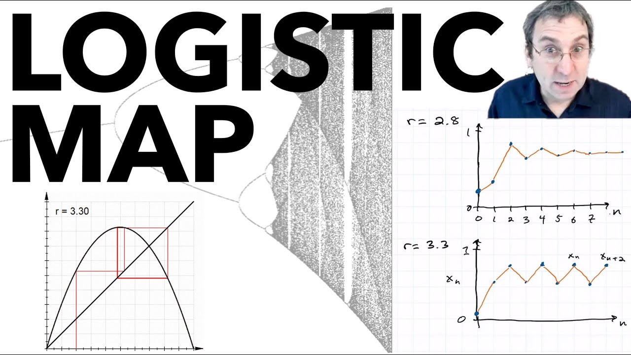
[00:00:04]this is a lyapunov fractal my hope is that by the end of this video you'll understand how these are generated what these colors mean and why it seems to overlap itself sometimes the oppanav fractals or marcus the oppanov fractals were first created by physicist mario marcus in the late 1980s they were popularized in the september 1991 issue of the scientific american magazine the fractals are named after alexander leoponov who laid the mathematical groundwork for them in his doctoral thesis in 1892 having died 104 years ago he never knew that this fractal among other things would bear his name so what does lyapunov have to do with this fractal how did marcus create them can it be generalized let's answer those questions in order we can't get very far into this discussion without talking about iterated functions or maps luckily it's a pretty simple concept pick a number which we'll call x naught now pick a function f of x now we run the number through the function the number has just been mapped to another number now we put the result back into the function and repeat okay let's try it with some actual numbers now we'll have an initial value of negative one-half and our function will be cosine i've also added a number line so we can see where we end up with each iteration so we start off at negative one-half then we go to 0.87 then 0.63 and so on the actual values aren't important what we're interested in is the behavior here we can see that it's kind of zeroed in on a point about 0.735 in fact for cosine regardless of the initial value the iteration sequence will always converge to this point let's look at another example with this function the output ends up bouncing between two points in a kind of cycle in another example the sequence rushes off the screen towards negative infinity and in one last example the sequence never converges to a number or settles into a cycle of numbers but it never blows up to infinity either it just bounces between seemingly random values this behavior feels chaotic doesn't it all right let's recap on the different kinds of behaviors we've seen we know that these sequences can converge to a single point end up in a cycle between several points blow up to either negative or positive infinity or chaotically bounce between points maybe it would help if we found a better way to visualize these iterative sequences but first let's pick one function from now on and stick with it the map that we'll be looking at for the rest of the video is the logistic map you may have noticed that this is the map i used for the last few examples in the previous section this is not a coincidence the lyapunov fractal is generated from a modified version of the logistic map so it'll be important to have a good understanding of it going forward now at the end of the day when we iterate through these maps all we're really doing is generating a list of numbers so let's plot them out over time now let's draw some axes and some lines connecting the iterates and we've got a plot we can still move x naught around but from now on we'll keep it here at one half also right now we're only looking at 10 iterates let's bump that up to 50.

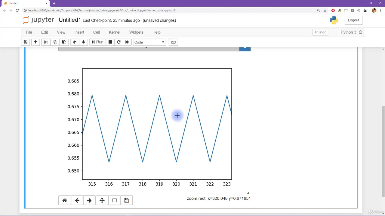
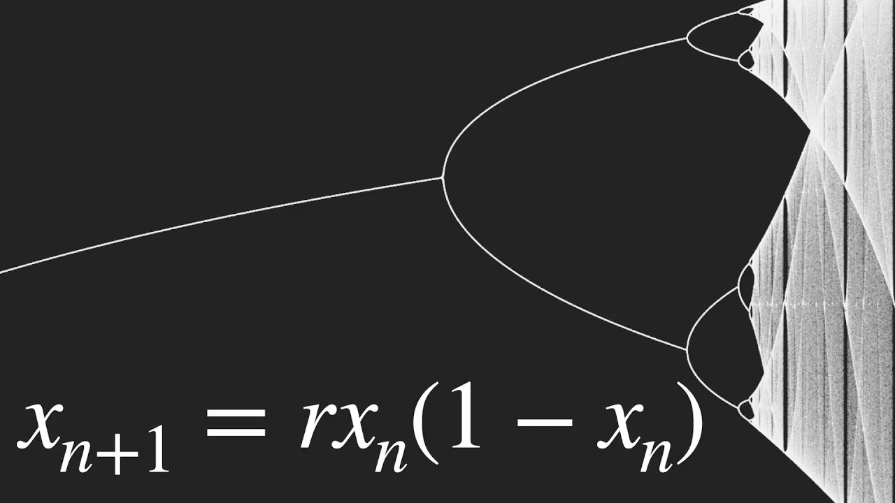
[00:04:16]what we're really interested in is not changing the initial condition but changing the function itself we'll do that by changing this r value i'll set r to zero and then we'll sweep through the values of r and see how it affects the plot okay well when r equals zero the iterations very quickly converge to zero as r is increased the iterations continue to converge to zero up until around r equals one note that it takes longer for the sequence to converge to zero here as we move past one instead of converging to zero the iterations converge to some other number depending on r the behavior changes again when r approaches three once again it looks like it's taking longer to converge to that point well if we go past three then instead of settling down on one point it oscillates between two points in a cycle like we saw before this splitting is called bifurcation let's keep going look at that it's split again and now it oscillates between four different points and now it looks chaotic and doesn't seem to repeat at all but now it's gone back to being stable maybe it'll continue to be stable from now on no it went back to chaos and when r goes above four even just by a little bit the sequence blows up to negative infinity maybe another plot can give us more insight a bifurcation diagram should help with that let me show you how to generate one i've introduced a new plot on the left which plots the final values of the sequence as r increases so again at first the sequence converges to zero then when r approaches one the sequence takes a lot longer to converge as we move on the sequence converges to some other point and as r approaches three it again takes longer to converge since it's starting to be pulled towards two different values as we move past three it bifurcates then bifurcates again then becomes chaotic then stable then chaotic again all right let's do that again but we'll trace out the path that those final values take this time this is the bifurcation diagram actually our r value can be negative too there this is the complete bifurcation diagram for the logistic map let me just change the colors and move those axes out of the way by the way the reason i'm restricting r from negative 2 to 4 is because outside of this bound the sequence just blows up to infinity like you've seen so there's really nothing out there to see let's go ahead and zoom in on this region here there's some pretty interesting things to see here we have bifurcations this general region of chaos and we have islands of stability within the chaos you know it would be pretty handy if we could simply look at an r value and tell if the corresponding sequence will be chaotic or stable well that's where alexander liapanov comes in he was the first to define stability in his phd thesis in 1892 and the method he created is now called the lyapunov exponent usually denoted with a lambda here's how you calculate it for discrete functions which is what we've been working with let's go through an example real quick first we need to find out how to calculate the lyapunov exponent for the logistic map specifically all we need to do is evaluate this derivative here all right so here's the logistic map if we calculate the derivative we get r times 1 minus 2 x sub n we plug that into the equation and there now we know how to calculate the lyapunov exponent for any sequence that was generated using the logistic map luckily we only have to do that part once now let's pick an r value we'll go with this one we saw earlier here's its plot of iterates we're going to use those iterates to calculate the correspondingly upon of exponent we'll start by running all these iterates through this function inside the summation block here's what we get all this part means is that we'll take the average of the results so when we do that we get oh hm this negative infinity is going to cause some problems the 0.5 at the beginning will always result in a negative infinity but since we're always going to start with the 0.5 we'll just skip it when we calculate the average there now we can actually get a result one other thing we're only using 10 iterates this limit here would like us to use infinite iterates to calculate the truly open of exponent that's asking a bit much maybe one million is a good compromise so what does this tell us about the stability maybe if we just plotted over all the r values we'll get some insight on the horizontal axis we have r and on the vertical axis we have lambda let's go ahead and plot their relationship well here it is it's certainly very spiky hmm it looks like lambda stays negative unless r is near the edge of the plot how about we take the bifurcation diagram from earlier and compare it to this plot perhaps unsurprisingly it lines up perfectly in many key places when there's bifurcations the lyapunov exponent is zero in between those bifurcations lambda spikes downward most crucially though as soon as the bifurcation diagram enters its chaotic region lambda becomes positive and where there's these islands of stability lambda spikes downward again below zero so when the lyapunov exponent is negative the system is stable and is attracted toward a point or cycle of points when lambda is positive the system is chaotic and doesn't settle on a point or cycle not only that but the magnitude of lambda measures how stable or chaotic the behavior is for instance when r equals 0 or 2 not only is lambda negative but it's negative infinity so those are called super stable points this means that the sequence very quickly reaches its final state where there's bifurcations and lambda equals zero the system takes an infinite amount of time to reach its final state speaking of infinity when r is less than negative two or greater than four lambda gets very large very quickly and races towards infinity all right now we know everything we need to know about the iphone of exponents and we can take a look at mario marcus's modified version of the logistic map basically his idea was that as you're calculating the iterates you switch the r value to a different r value and then you alternate between them so from now on we'll have two r values for each list of iterates we generate let's go ahead and pick some 3.2 and 0.7 having two numbers called r is kind of confusing so let's rename them a and b great let's use them to calculate some iterates once again we start with an x naught of 0.5 which i've colored gray when we generate our first iterate our r value will equal a which is 3.2 colored red when we calculate our next iterate we'll use 0.7 or b as our r value this one is green then we repeat indicated by this dashed line each red iterate was calculated when r was equal to a and each green iterate was calculated when r was equal to b as you may have guessed we're interested in the behavior of this sequence even though we're alternating between r values the system still gets trapped in a cycle we have a few ways of affecting the iterates for one we can change the values of a and b the other thing we can do is change how r alternates between a and b for instance instead of just going a b and repeating we can do a a b then repeat or a b b a or six a's then six b's or whatever other sequence of a's and b's you'd like of course we can calculate the lyapunov exponent for any of these sequences let's take a step back first though and think about all the new inputs we have before with the original logistic map we were mainly concerned with changing r and seeing how that affects lambda which tells us how chaotic the sequence of iterates is depending on r with the modified version we're doing the same thing except r is now determined by a b and s s being our sequence of a's and b's that tells r how to switch between a and b all right now let's do some plotting here we have the a b plane each coordinate on this plane represents a pair of a b values let's start with this corner here which corresponds to a equals four and b equals zero i've also set our sequence s to a b for this coordinate lambda equals negative infinity this means it's super stable we can color this coordinate based on the correspondingly open up exponent remember that if lambda is negative the system is stable and if it's positive the system is chaotic we can create a color scheme based on that information we'll color stable coordinates yellow and chaotic ones blue so this one for instance will be yellow let's look at the next one a equals four and b equals one this coordinate results in a positive lambda so it'll be blue now let's go ahead and fill in the rest of the plane we can do a couple things to make this look nicer the most obvious thing to do is to increase the resolution first though we'll modify the color scheme we'll have the stable side go from black to yellow as lambda goes from negative infinity to zero this means the more stable the sequence the darker the yellow on the chaotic side the color will go from blue to black as lambda goes from zero to infinity so the more chaotic the darker the blue now let's fill out the plot now this is much better than that flat blue and yellow let's double the resolution now and let's double it again as i increase the resolution i have to lower the number of iterations so i can generate these in a reasonable amount of time anyway what we're left with is the lyapunov fractal these dark bands indicate coordinates of a and b that generate a sequence of iterates that are very stable the lighter bands correspond to sequences that are less stable or a bifurcation happens around there the blue areas are of course chaotic now we don't have to use this color scheme but it's one of the ones that mario marcus originally used so it's sort of the default now that we're here let's explore a bit i know it's kind of hard to tell the scale which i suppose is a property of all fractals but here let me turn on some grid lines again b is horizontal and a is vertical each one of these boxes is one by one on the coordinate plane this point is 2 2 and this point is 4 4.

[00:17:15]with that in mind let's zoom out the black region surrounding the fractal is where the iterates generated by a and b race off to infinity so lambda is also infinity this point is the origin when either a or b equals zero the iterates very quickly converge to zero so lambda is negative infinity anyway like any good fractal we can zoom in to see arbitrarily small details i'm rendering this fractal pretty quickly but the cost is a lack of precision so i can't zoom in too far so far we've only been looking at a b let's look at some other sequences hey wait a minute this one looks like the first one we saw hmm this one's ba let's compare it to a b again yeah look at that if you switch the order of a b it changes which branch is on top let's see if we can find an explanation for what's going on here okay i've put the two fractals side by side let's take a look at a particular a b coordinate which i'll mark on these plots with this black dot i chose this coordinate in particular because it's in the area with the overlapping branches when our sequence is a b the lyapunov exponent for that point is negative 6.96 and when the sequence is ba lambda is negative 0.36 let's take a look at the iterates for the fractal on the left the sequence ends up in a two cycle the one on the right though ends up in a four cycle even though both sets of iterates have an r value that swaps between 3.3093 and 3.5 the behavior of the iterates is not the same it depends on where in the sequence s we start here's another example basically my understanding is that if you have a sequence of a's and b's of length l the resulting iterations can have up to l different behaviors depending on where in the sequence you start which means up to l different possible the output of exponents for any coordinate a b if you start at a different point in the a b sequence then different branches will be on top like we're seeing here with these three fractals for this a b coordinate the iterates can have one of three different behaviors and thus can have one of three different lambda values depending on if the sequence is aba baa or aab let's backtrack a bit and revisit the bifurcation diagram it can be extended from the logistic map to this modified version in the original bifurcation diagram the horizontal axis was r and the vertical axis was called x which maps the values that the iterates end up with given r well now we essentially have two r values so that adds an axis to our plot here it is just like in the 2d version we have this large region of chaos where both a and b approach 4.

[00:21:14]here you can see bifurcations let's look at it from above it looks a lot like the fractal doesn't it let's compare we can see a lot of similarities between these like i've mentioned these white lines where bifurcations happen and now you can see how they happen in the bifurcation diagram you can also see patterns of lines that are analogous to these dark lines of super stability you can even see the branch overlap in the bifurcation diagram and if we switch to ba you can see the other branch here's something to consider this diagonal line along the fractal is where a and b are equal so even though our r value switches between a and b since they're the same it's equivalent to having just one r value so marcus's modified logistic map is equivalent to the original logistic map when a equals b we can especially see this when we line up the 2d bifurcation diagram along the a equals b line once again things line up in very convenient places since a and b are equal here i'll just call them r when r equals one there's a change in the behavior of the bifurcation diagram so the lyapunov exponent is negative but close to zero which is what this white band represents the first bifurcation in the diagram at r equals three matches the place where the branches start to overlap in the fractal and at about r equals 3.83 there's an island of stability it's covered by the axis right now so here's another view of it on the fractal anyway all the oppanof fractals have this relationship with this bifurcation diagram along this line here's another example we've looked at 3d bifurcation diagrams but the fractals themselves can also be extended to 3d all we have to do is add a new letter to the sequence there now there's a c which adds a whole new dimension to explore you could render the 3d fractal as an object in 3d space but we're going to use c as a time axis that is to say we'll be looking at 2d slices of the 3d fractal and that is exactly what you saw at the very beginning of this video there is one other thing we can do to generalize this fractal we've been using the logistic map this whole time but you can use other maps each map has its own bifurcation diagram and fractal again any fractal you want given a sequence of a's and b's i'll cycle through some here at the end thank you so much for watching you