



























The logistic map, defined by the recurrence relation x(n+1) = r*x(n)*(1-x(n)), demonstrates a period-doubling route to chaos as the growth rate parameter r increases: stable fixed points bifurcate into period-2 cycles at r≈3.0, then into period-4 cycles at r≈3.45, followed by period-8 cycles at r≈3.54, and so on, with the bifurcation points converging geometrically toward an accumulation point r∞≈3.56995; beyond this point, the system enters chaotic behavior characterized by sensitive dependence on initial conditions, yet periodic windows persist within the chaos, including period-3 windows at r≈3.8284, demonstrating that even simple nonlinear maps can exhibit extraordinarily complex dynamics.
Logistic Map: Period Doubling Route to Chaos | Nonlinear Dynamics
Added:The concept of discrete dynamical systems and iterative functions (specifically systems defined by x_n+1 = f(x_n))
How to find fixed points and evaluate their stability using derivative-based stability criteria
Familiarity with cobweb plots (cobweb diagrams) to visually track the orbit of a discrete system
An introductory understanding of population growth models, particularly the distinction between exponential and density-dependent growth
Feigenbaum scaling and the universal Feigenbaum constants that govern the rate of period-doubling cascades
Lyapunov exponents as a quantitative measure of a system's sensitivity to initial conditions (the 'butterfly effect')
The transition to continuous-time chaotic systems, such as the Lorenz equations and Rossler attractors
Fractal dimensions and the geometric structure of strange attractors (e.g., the Cantor-like structure of the logistic map's attractor in the chaotic regime)
Real-world applications of chaos theory in meteorology, cryptography, cardiac dynamics, and financial market modeling
15.6K views266likes17:18Original Release: 2021-04-20
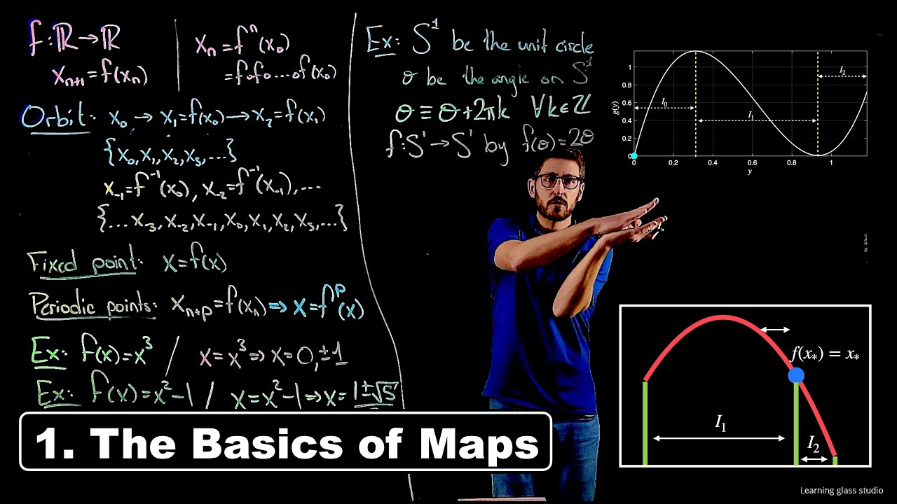
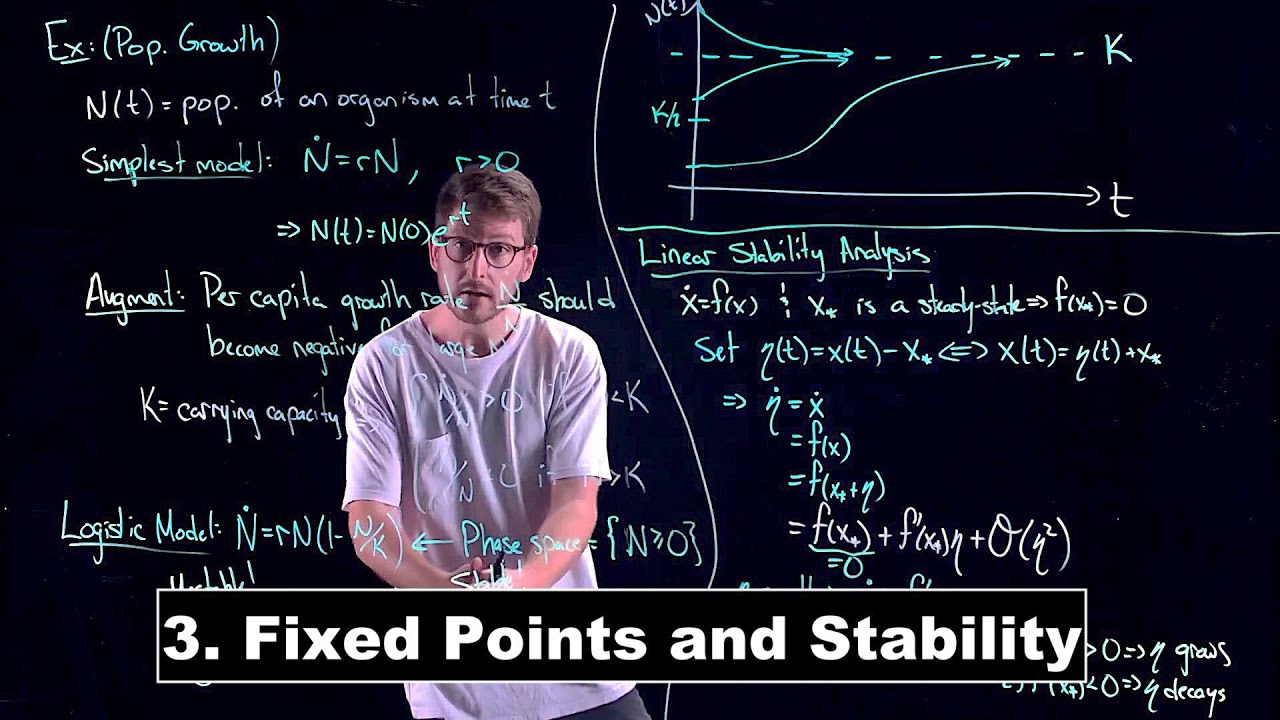
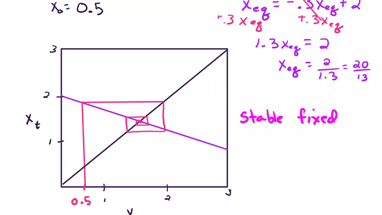
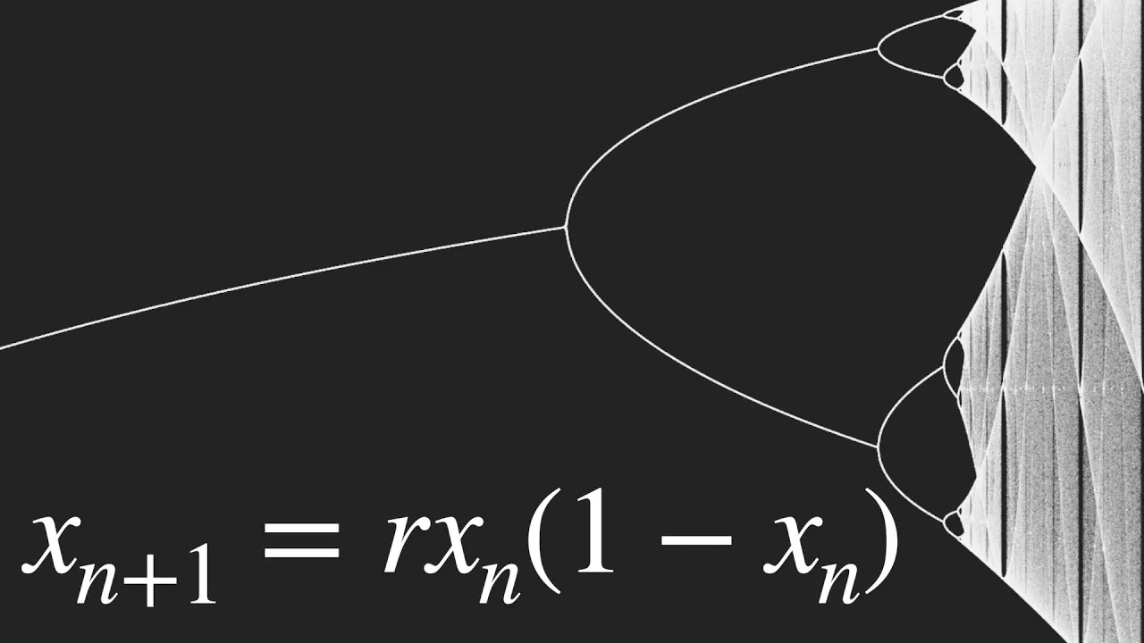
The thing that I'll be talking about today is the logistic map and it's really simple--it's like shockingly simple. So this is just 1d, we say x n plus one is r that'll be a parameter we could vary x n times 1 minus x n this was created to be like a discrete population dynamics model similar to the logistic equation if you remember the logistic equation that was a differential equation but it had a right hand side that looked something like this where there was like a carrying capacity for a population but here the space of x we're normalizing so that it just goes from zero and one so we're talking about the interval zero to one what is r if you were to plot this you can plot x n plus one so this is a bit like if you remember the graphical method for one dimensional differential equations well here we're plotting the map there's zero there's one so here's x and everything has to be between zero and one we're only allowing between zero and one where does this peak it actually peaks at the halfway mark so one half it's a parabola goes up from zero and then it goes back down to zero symmetrically and it peaks at r over four we want the map to go from zero to one to zero and 1. so we want x n plus 1 to be somewhere inside the unit interval and for that to happen we need that this peak be 1 or below so it's conventional to let the parameter be something less than four but greater than zero and physically this is supposed to represent the reproductive capacity of the population it was first in a paper by robert may 1976 in nature it has some interesting name simple mathematical models with very complicated dynamics and it's now become a classic he talks about first order and he called them difference equations and maybe that's a term you've heard or used in addition to iterated map or i think recursion relations are also used so he wrote this right and that's what we're looking at he called the parameter a and referred to time the discrete time as t we're going to refer to the discrete time as little n and use r as our bifurcation parameter robert may uh was a i think trained in physics but then was in biology departments and was sort of a father of uh ecology so it's become this classic this is where the logistic map was introduced in some sense it's the simplest non-linear map because all it has is a quadratic non-linearity xn plus 1 equals if we were to write it out it's r x n minus r x n squared if it was just r x n then it'd be a linear map easier to analyze but it's non-linear what happens what's the big deal with this map you can pick an initial condition x naught which has to be somewhere in this interval between zero and one and then you would write you know x one equals r x naught one minus x naught and then you'd say well x two whatever you get for x one right so this is it's really simple to code up as a for loop and then plot it r x one 1 minus x1 and so on and then you can just see what happens so we'll do that for some initial conditions i'll sketch some here but then we'll even see it numerically it's you could pretty easily find numerical tools online for the logistic map because it's it's so well known the parameter is going to play a big role bifurcations are very important here if we were to look at what happens with r equals 0.5 along this axis the horizontal axis this will be the discrete time n so it'll be times zero and the interval over here will be i'll be plotting x n has to be between 0 and 1. it turns out for any initial condition for 0.5 you would get something like this so here's our initial condition and then this will just get lower and lower and lower and really the map only spits out these points x n goes to zero for any x naught so any initial condition as n goes to infinity so x equals 0 is a fixed point of the map you might put it that way at least for this value of r now sometimes people will connect the dots but that's just to guide your eye the map only spits out points but if i wanted to guide your eye i would draw straight segments between these and you can get an idea of what's happening right and you could demonstrate that it goes to zero we could think of this also in terms of the cobweb plot if you remember the cobweb plot where we write x n x n plus one we draw the diagonal 45 diagonal line let's call this one that's one and this is zero zero for r 0.5 this thing rises to only the level of what r over four so that's 1 8. so it's not going to be very high it's going to be it never actually other than at the origin it does not intersect that 45 degree angle line so according to the cobweb plot construction if we started with some initial condition we would go up to the curve and that tells us where to go we go from there horizontally to this 45 degree line and then this would take us down to this point i kind of have to zoom in here oh look at that look what i can do and then we would go across to here and you can kind of see the cobweb plot is just taking us into the origin and this would this will happen no matter where we start so i'm just using the same rules for the cobweb plot that i did before when we were talking about the lorenz map so that's for r equals 0.5 what about for something a bit bigger so i'll look at r equals 2.8 this is what we get for the the orbit if we start somewhere i'll start at some other initial condition remember this only goes from between zero and one if i start say here the next iterate gets a little bit further up and then i go up somewhere but then i go down and that just sort of dampens out until i reach a fixed point and again the map only spits out the points we could draw lines to connect it to guide your eye and you can see hopefully what's happening it looks like it overshoots but then it eventually settles down to a fixed point that's non-zero x n goes to x star as n goes to infinity and x star is not zero so there's some non-zero fixed point that shows up and it's the same x star for any initial condition and remember the the range for r we said it's conventionally taken to be from zero to four and i'm picking these strange values what about r equals 3.3 we do the same kind of diagram so this is xn it goes between zero and one here's what we would find start with some initial condition what we would get is that this will go up and eventually it'll settle down on a cycle so it's going between two points over and over again so this is like the discrete map version of a limit cycle instead of being a fixed point we settle onto a a cycle you know it jumps between the same two points now as n goes to infinity and this is independent of the initial condition so you take any initial condition it'll it'll settle on this we call this a period two orbit or you could call it a period two cycle and it's also stable it is the attractor it's the attractor because an open set but actually every initial condition ends up there and you get this repeating so x n plus two equals x n as n goes to infinity right if this is x and then it's just going between the two so that's interesting what if we turn this knob a little bit higher r equals 3.5 we get something that settles on a a cycle but it settles on something where it goes down and then up and then down and then higher and then it repeats that down up kinda down up it's a lot easier if i connect points and maybe even zoom in so it's repeating but it's not repeating every two iterates it's repeating every four iterates so we would call this a period four cycle so that's interesting what happened to three we had in this case we had period doubling and period doubling will be sort of one of the main phenomena that goes on here you can find these numerically some of them you can find analytically but think of just you tune r and you look for the value of r where a stable two to the n cycle first occurs as we turn this knob even further we'll go from a period 4 cycle to a period 8 period 16 and so on and i'll call the special value of r i'll call it rn it's the value of r where a stable 2 to the n cycle first occurs so it turns out if you notice what we had up here at least for r 2.8 we didn't have one it was just a fixed point for our 3.3 we did have a stable two cycle so that means two to the one so r1 that happens at three and that can be shown so a period two cycle is born r2 occurs at so that would mean a two to the two cycle or four cycle three point four nine if we keep continuing this r3 is at 3.54409 so that's a period 8 cycle 2 to the 3 is 8.
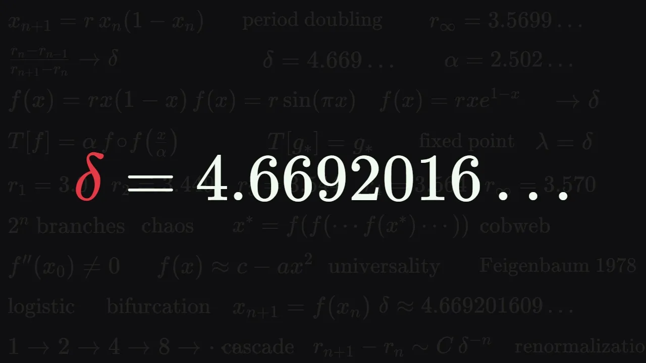
another period doubling at three point five six four four and so on what is going on with this sequence it's looking like it's converging to something so r to the five that would be where there's a 32 cycle is 3.568759 looks like it's converging to something close to like 3.5 7. it actually is so if we were to look at what's going on r n converges essentially geometrically to some point called r infinity which robert may in the paper refer to as the accumulation point if we were to sketch the interval this is r we could draw r1 and everything at this point this is let's call this the accumulation point everything's going towards r infinity so here is say our n here's our n minus 1. so we have that the length of that first gap between the values the next value rn plus 1 is a smaller gap and the gaps keep getting smaller and smaller and it's kind of hard to draw but it all accumulates at that point or infinity if you look at the ratio of rn minus r n minus one so that kind of the longer gap divided by the size of the smaller gap as n goes to infinity the ratio of those gaps becomes a fixed number 4.6692 something something something and we'll say more about what that number is right now let's just say it's a it's a mystery it's sometimes called delta but that's what's going on r infinity is something really close to 3.57 there's still plenty of room between r infinity and four so you might wonder what's going on there actually a shocking amount of stuff happens so what was drawn what's been drawn and it's now become a pretty famous diagram is to plot something like a bifurcation diagram it's not technically a bifurcation diagram but it's often called a bifurcation diagram so we're plotting r and what did we so what do we have up here we're plotting x n on the attractor so we're plotting all the points on the attractor so what have we shown up above uh well for 0.5 we were at zero so this only goes between zero and one 1.
this is what's happening at 0.5 right we just we were at 0. in fact we stay at 0 until the value 1 and at the point one zero still is a fixed point it's an unstable fixed point so we might draw that as dashed what we really care about is where the points are there's the branch that shoots off we looked at 2.8 and that's just a point it's just a fixed point but then at three this bifurcates into two branches so if you remember where we were at 3.3 this isn't going to be completely to scale but we had two points there's actually a branch coming off that fixed point that goes between those two points there's still an unstable point but it's unstable so you wouldn't observe it so it's usually not depicted in this thing that would be called the bifurcation diagram of the logistic map at 3.5 we had four points and that's because somewhere in there was r2 and that's where there's a splitting again we call this the period doubling and this period doubling keeps happening at each of those values of rn so it's it's hard to depict so i zoom in here where were we 3.5 i think so there's more and more splittings you could just think of there being little it looks like a tree with branches and eventually there's a r infinity you hit r infinity and all these branchings just go into a mess of chaos i'll just show what look like tons of little branchings and then we have chaos and i don't even know how to draw it but it you know you'll just have points all over the place not actually all over the place but somewhere and then here's the weird thing there's a window later on there's several windows there's an infinite number of windows but there are big windows of going from chaos back to periodic behavior this is depicting chaos and then we have periodic window and the kind of biggest periodic window has period three that shows some period three orbits those branch and then there's chaos again and then there's windows this diagram is an intermingling of chaotic and periodic windows this was surprising why would such a simple map in some sense the simplest non-linear map shows such rich behavior but there it is it's real in fact this point where the kind of biggest periodic window shows up occurs at one plus two square root two which is about three point eight two and that's where the period three stable attractor was born it turns out you can find attractors of any period so give me any integer for some parameter value there will be an attractor that has that period because in this region that i've called chaos there's actually periodic windows inside there they might be infinitesimally wide but they're there there's a lot to unpack here and try to understand
Up Next
47:11
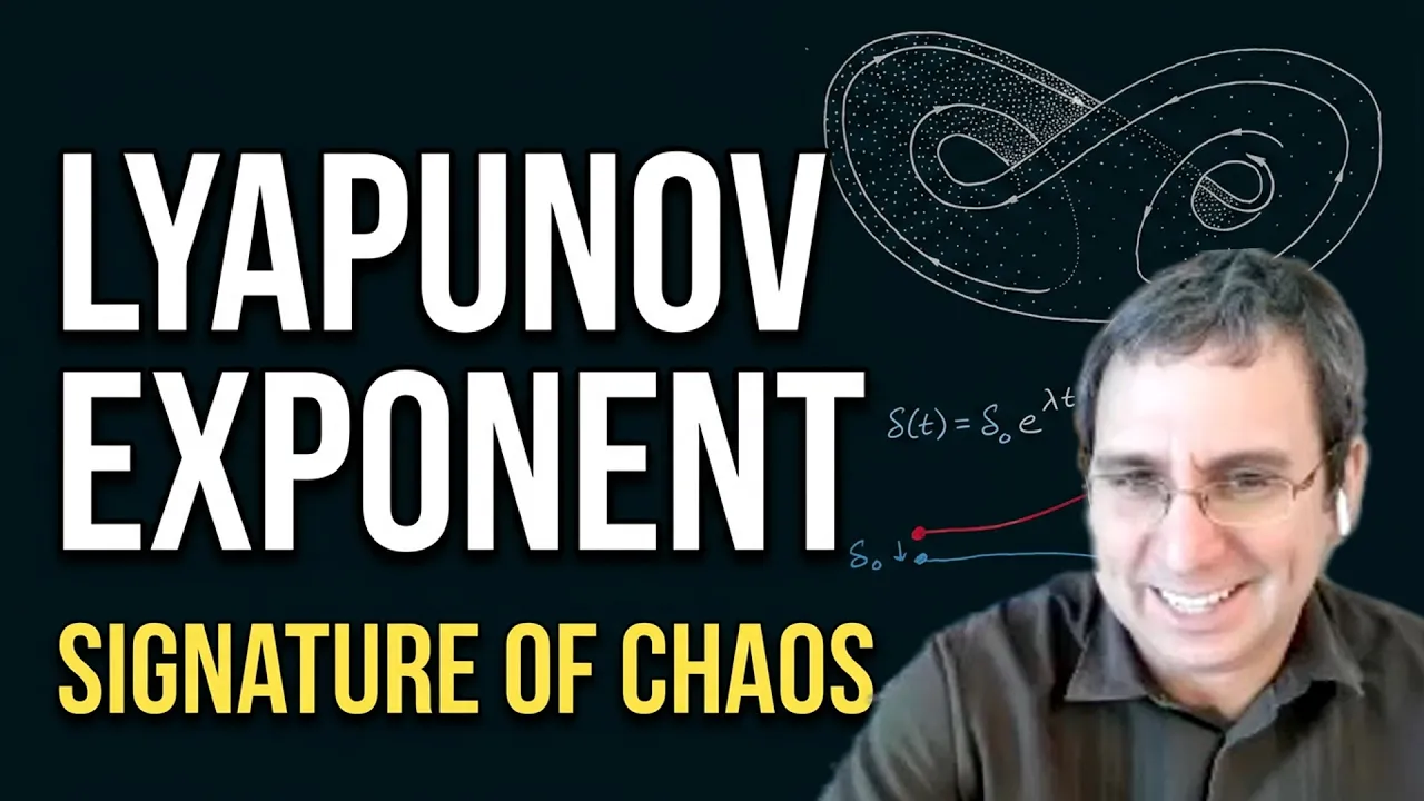
Feigenbaum Constants, Lyapunov Exponent, and Renormalization
@seyjah
328 views•2024-04-25

4:43
Elliptic Curve Cryptography Explained: ECC, ECDSA, ECDH
@PracticalNetworking
28.5K views•2024-10-21

10:44
Fourier Series Introduction: The Big Idea Explained
@DrTrefor
387K views•2021-05-03

6:00
The Mathematical Impossibility of Accurate World Maps
@Vox
23.3M views•2016-12-02
Related Study Plans & Knowledge Roadmaps
Structured learning paths in Mathematics
mathematics
Tensor Calculus: Vectors to Riemann Curvature
01Mathematical Foundations: Linear Algebra & Calculus
02Covectors, Dual Spaces, and Tensor Basics
03The Metric Tensor and Index Gymnastics
+ 2 more learning modules
40h5 modules
Explore Roadmap
mathematics
Gödel's Incompleteness: Logic, Proofs & Limits
01Introduction to Formal Systems & Hilbert's Dream
02Set Theory, Cardinality, and Cantor's Diagonal Argument
03Arithmetization and Gödel Numbering
+ 2 more learning modules
14h5 modules
Explore Roadmap
mathematics
Galois Theory: Fields, Groups & Solvability
01Foundations of Abstract Algebra: Groups & Fields
02Polynomials & Field Extensions
03Splitting Fields & Symmetries
+ 2 more learning modules
24h5 modules
Explore Roadmap
mathematics
Non-Euclidean Geometry: Models & Geodesics
01Euclid's Fifth Postulate and the Birth of New Geometries
02Hyperbolic Space and the Poincaré Disk Model
03Geodesics: Defining Straight Lines in Curved Spaces
+ 2 more learning modules
15h5 modules
Explore Roadmap