





![Stability and Eigenvalues [Control Bootcamp]](https://i.ytimg.com/vi/h7nJ6ZL4Lf0/maxresdefault.jpg)


















![카오스 이론은 우리의 미래를 예측할 수 있을까? [북툰 과학다큐]](https://i.ytimg.com/vi/A79HPtXfQMY/hqdefault.jpg)

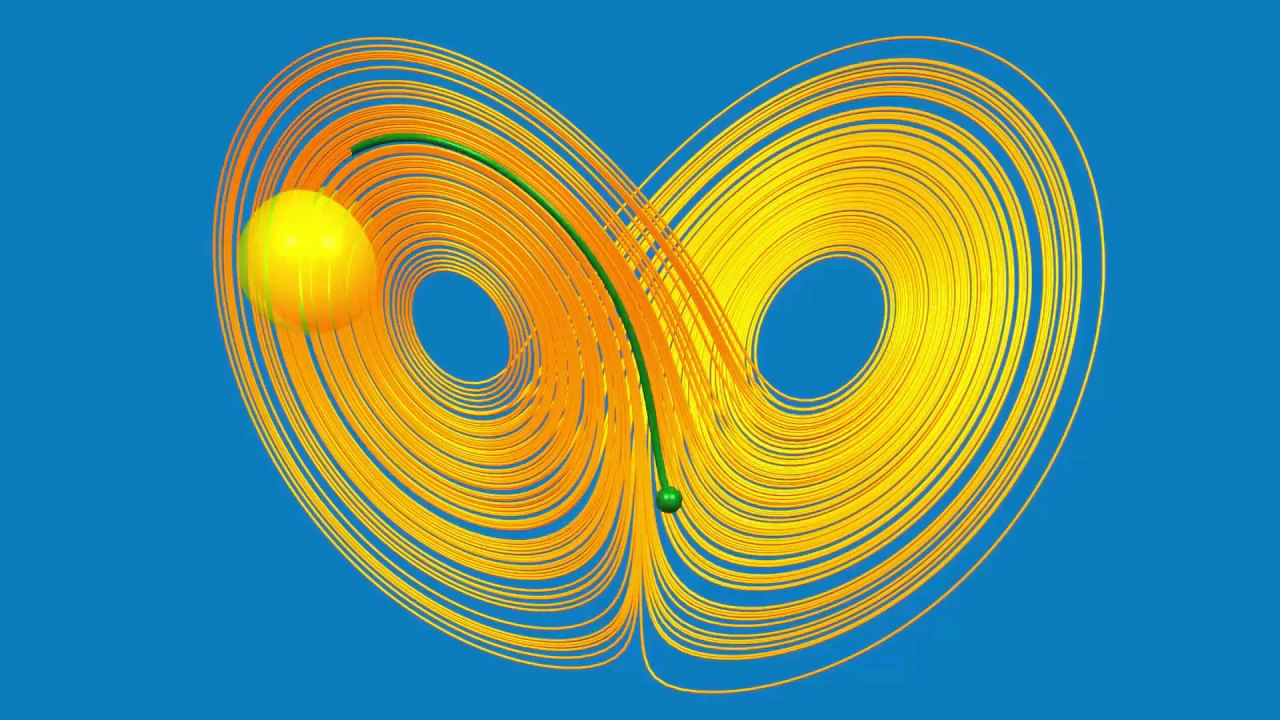
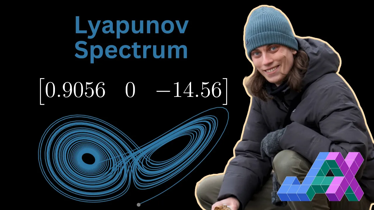
Sensitivity to initial conditions, often called the butterfly effect, is a fundamental property of chaotic systems where small differences in starting points lead to vastly different outcomes over time. This sensitivity is mathematically quantified using Lyapunov exponents, which measure the exponential rate at which nearby trajectories diverge. The maximum Lyapunov exponent (λ_max) determines whether a system exhibits sensitivity: if λ_max > 0, the system is sensitive to initial conditions; if λ_max = 0, it is neutral; and if λ_max < 0, perturbations decay exponentially. Importantly, sensitivity to initial conditions is necessary but not sufficient for chaos—linear systems can also exhibit positive Lyapunov exponents without being chaotic, as they lack the other components required for true chaos (topological transitivity and dense periodic points).
Understanding Chaos Theory: Lyapunov Exponents & Sensitivity
Added:okay welcome back everybody moving on to one of my favorite sections in the book you know we're kind of concluding it in many ways but these these last few sections really are my favorite they've been working really hard to give ourselves a tool so we can handle some of these these Arcane topics such as chaos and so today's the first really our first day on chaos and in particular the subset of chaos that we're going to be studying today is this so-called sensitivity to initial conditions um a lot of you probably have heard of this as the butterfly effect and the mathematical term that we often use to describe a sensitivity to initial conditions is leapuna of exponents so there's another fun name for everybody to memorize liabenov Alexander the abanov he was a I believe Russian math Edition in the early 1900s and he had a lot of really really good things to say about chaos and really Dynamics in general um as well as stability so actually we could have we could have taken a lyapanov approach to stability in the previous section but we didn't anyway here we're stuck we have to take the Billy up and up approach and uh before we get into it too much let's talk about chaos as a whole and chaos and continue continuous time Dynamics my definition this is something that's important to recall is that the method the mathematics Community as a whole doesn't have a definition that everybody agrees upon but a very common one is is a definition by a man known as devaney definition and uh devaney's definition is the one that we're using here as well and so this definition of chaos has applied to a continuous time Dynamics is we're going to start with the continuous time Dynamics and we can initialize it anywhere but we say that this exhibits chaos we can also use chaotic Behavior or is a chaotic Dynamics and it's allowed to exhibit chaos only in a region right so we're not requiring that this thing is fully chaotic everywhere we're allowed to to restrict ourselves to a region and say it's chaotic within some region Omega if within that region we're sensitive to initial conditions which is kind of the section of or the the idea of this section and I've linked to the definition there we are topologically transitive and that's going to be in the next section section 13.3 within Omega and then we contain dense within Omega periodic points and that's also going to be in section 13.3 so two and three we're going to save to section 13.3 but uh number one which is maybe the most excited part about chaos it's the one that a lot of people think about this sensitivity to initial conditions that's going to be in our current section uh 13.2 and in particular we're going to try to Define this thing called the lyapanov exponent which is what what we really need to have a sensitivity like this well anyway to kind of head into the rest of these sections and actually the rest of the rest of this book is the following definition so I really want all of you to take a good amount of time to figure out what this definition is saying because the rest of the book relies very heavily on this definition okay so this definition is the definition of a flow map okay sometimes we'll just call it a flow that's a little bit ambiguous it may be a bad way to talk about it because it is a map it's mapping the flow but what it is is it's a it's a function and actually it's a vector field okay because I'm starting with a vector and I'm ending with a vector a d dimensional vector and it's parameterized by time greater than T naught okay so that's why I'm putting a subscript T comma T naught by it you'll see a lot of different notations for this sort of flow usually they're all similar you'll either have Phi to the power t or a v subscript T and A lot of times people will omit they'll omit T naught because they'll just initialize at zero okay so if you put a zero in there a lot of people just omit T naught for that but because I want to be a little general just say we can initialize anywhere I write Phi sub T comma T naught to say okay where are we initialized where are we now that's kind of the idea of TNT naught um and it's so it's a vector field so it takes in x a vector and it outputs a vector as well in this Vector so the vector output at time T the vector output at time T is is Y where that specific Y is actually the solution to my Dynamics initialized at X okay so whatever Vector I'm plugging into the flow map that's the initial point of the Dynamics and then I basically say okay my Dynamics is allowed to push me somewhere at time T if I wait you know 20 seconds my Dynamics pushes me somewhere and then I say wherever that's pushed me that's the output of the flow map so more or less the flow map is just a reinterpretation of this Dynamics where let's say it's a reinterpretation of Dynamics where the variable is the initial condition and in particular the initial spatial condition right let's say spatial so it's a reinterpretation of the Dynamics where my my variable which goes into the flow map is the initial condition of my Dynamics and then the parameterized part of my flow map is the time that I've waited so maybe I fix the time 30 seconds I say there's a map that takes me from an initial condition to wherever it ends up after 30 seconds let's say perfectly well defined map from a vector to a vector and so let's look at the next Dynamics here this is a nice example of just you know a single dimensional non-linear Dynamics and you'll notice that I've decided to initialize at X here and that's because I'm going to construct the flow map to this right so the way we construct a flow map by solving the Dynamics for an arbitrary arbitrary initial condition that's how we're gonna so if we solve this we end up with well traditionally we would solve it and we would say that this is y of T it's the solution to the Dynamics but you'll notice that when I write it like this if I write it as a y of T I'm emphasizing that time is my variable the flow map is the understanding that time is now a parameter and actually the initial condition X is the variable so that's all the idea is the flow map is reinterpreting the initial condition is the variable of the map so that's how I find my flow map you can verify it here right by actually Computing the time derivative and then you'll notice that it solves the the IDP okay but why do we care about a flow method at least in this section there's lots of reasons why we care about the flow Maps they're going to be one of the most useful tools in in the study of non-linear Dynamics for the rest of our book but why we care about it for this section is that we can actually think about okay suppose I initialize my Dynamics at X1 and I initialize my Dynamics at X2 then the difference in the flow maps for some time some future time T that difference describes the distance between the Futures right I can compute the kind of the spread this is the spread of X1 and X2 over time so that difference describes the spread of two initial conditions over time we can think about saying okay what about the spread of two initial conditions infinitesimally close to each other if I think about the spread of two initial conditions infinitesimally close to each other actually we can compute what that is an infinitesimal by just Computing the Jacobian right the Jacobian matrix of this flow and we get away with that because now it's a vector field right we can compute uh derivatives in space because we're interpreting this as a function of space and so we can we can compute the spread of two initial conditions infinitesimally close by really it's the Jacobian right but then it's acting on okay that's the direction of the spread rate DX is the the direction of infinitesimal spread so I look at the Jacobian of my flow map at some time T and I act that vector or that Matrix on the vector which describes infinitesimal spread and I recover actually what how the spread would evolve over time of two points infinitesimally close to each other now you can probably see where I'm going right because if I have some notion for which two points infinitesimally close to each other spread really far apart that's precisely uh sensitivity to initial conditions right if I if I think about if two points infinitesimally close to each other infinitesimally close spread a lot then I am sensitive to those I'll say that even to that initial condition right because I'm sensitive to this point x that point x is really sensitive because even if I'm infinitesimally close to it and I'm somewhere else though I'm just like pushed off of it an infinitesimal amount if the spread of those two x's is Big over time then that's what sensitivity to initial conditions is it's basically saying okay I start here I start really close to it but maybe the flow takes me in that direction for one of them and in that direction for the other if I have flows like that that's what it would be to be sensitive but then let's think about maybe quantifying this right so to quantify this we need to understand the Jacobian we really want to understand this Jacobian of the flow somehow and we can understand it using this this specific Matrix valued initial value problem so here I have a matrix valued initial value problem and it says that that the time the temporal change of this Jacobian which is a matrix is equal to actually the Jacobian of n where n here is the end from my Dynamics scrolling all the way up here right the N is the n on the right hand side of my Dynamics the non-linear term and I'm going to take the Jacobian of the non-linear term and I'm evaluating it at the flow okay so this is the Jacobian Matrix of non-linear n in Dynamics y Prime equals NY at t 0 equals y zero so it's that N I take the Jacobian but I evaluate the Jacobian evaluated at C sub T comma t 0 of the flow okay and then that's a matrix which acts on my Jacobian of my float okay so this is saying that the time change of the Jacobian of the flow is actually the Jacobian of n evaluated at the flow acting on The Matrix which is the Jacobian of the flow and in fact I initialize at the identity Matrix okay so this is an IDP which really easily describes the behavior of the Jacobian of the flow now unfortunately this ivp isn't terribly well defined because if we don't know this if we can't solve for this it's not easy to solve the IDP and in fact this is a nicer Mark in fact if we could solve for Phi sub T comma t 0.
of X then we could just compute d c d d 0 directly okay so Y is y is this equation even useful well sometimes you might have some bounds you can place on that Matrix and if you have some bounds you can place on that Matrix then you can solve this equation at least in some bounded sets and so you can talk about qualitative properties of the Jacobian of the flow without necessarily having to uh to solve for the true flow and so that's why this equation is actually useful I have a proof of it the proof is not terribly difficult you just kind of re-represent the flow and take a Jacobian of it all right so now we have this idea of the Jacobian of the flow and now we're almost ready to get to the point of sensitivity to initial conditions we have this notion of the lyapanov spectrum so this is probably the most important definition you can memorize from this section aside from the definition of the flow because the lyophonous spectrum is how we're going to verify this is how we verify sensitivity okay so we verify sensitivity by constructing a matrix which we call Lambda sub X Lambda I believe for liabinov sub X for it's specific to a point at which you start and and this Matrix is going to be the limit at Infinity of the Matrix logarithm where you know jump back to chapter two to recall how you calculate Matrix logarithms with you know Jordan form Etc so jump back to chapter two for that so we're going to take a matrix logarithm of the Jacobian of the flow transpose multiplied by the Jacobian of the flow and then we're going to divide that matrix by 2T and take T out to Infinity that's going to be called The lyapanov Matrix and the spectrum of that Matrix which I recall that a spectrum also from chapter two the section relies on chapter two a lot Spectrum equals Sigma equals the set of eigen values okay so I'm just going to compute all of the eigenvalues of the Matrix that set of eigenvalues is my spectrum and if my Matrix in particular is this Matrix then I have what I call the liabinov Spectrum okay and that leoping out Spectrum starts at X because actually these flows are supposed to be on X here so those flows are flows on on the the initial condition X so let's look at maybe calculating one of these in in a one-dimensional setting right this Matrix will just be a one by one Matrix and so things get a little bit easy but we'll go ahead and do it and so we'll calculate the lyapanov Spectrum for this Dynamics y Prime is y squared and we initialize at X and we've already seen today that the flow map and I dropped t0 there because I'm initializing at zero we've already seen that the flow map is just x divided by 1 minus x t which means taking a Jacobian in one dimension is just a partial derivative with respect to X that Jacobian take a partial derivative with respect to X we have the following right and so now to calculate the lyopanov Spectrum now that I have this when you have the Jacobian of a flow the lyapanov Spectrum recall is I'm going to take the limit as T goes to Infinity of the log of the transpose of the Jacobian times the Jacobian divided by 2T and so I'm going to take that I'm going to transpose it but we interpret right so interpret this as a one by one Matrix so for a one by one Matrix it is its own transpose so basically I'm multiplying it by itself so I'll square it I'm going to take the log of that function squared and I'm going to divide by 2T so there we go there I have it I take the log of the function squared and I divide by 2T if I simplify that the two with properties of logs my 2T can come over here as a 1 divided by exponent so I'm going to be taking this to the 1 over T power one more log rule pulls out a negative 2 and I actually have 1 minus x t to the 1 over T now this is maybe a little unclear how we would compute the limit as T goes to Infinity of this but jumping back to the first time you encountered e in fact the first time you encountered e you encountered it probably as continuously compounded interest and you saw that the limit as n went to Infinity of 1 plus X over n to the nth power was e to the negative X or e to the positive X and then if I just put a negative sign in front of X I get e to the negative X and that's actually What's Happening Here with this limit and so we're getting a negative 2 times the log of e to the negative X which ends up being the log and the E cancel let me get 2x out of this okay so 2x is our lyapanov Matrix this is Lambda sub X as a matrix a one one by one Matrix but the spectrum of a one by one Matrix is just the number itself right and so that spectrum is 2X and so I have the up enough Spectrum for this Dynamics and I've calculated it as 2x we can then add an extra condition onto our our spectrum and this is called the maximal or top lyapanov exponent and it's simply the maximum value within thely up and off Spectrum so we're just looking at the Top Value in the up enough Spectrum and why that's important is that this next remark refers to the fact that the opinion Spectrum represents a rate of exponential spread so if I have two points infinitely close together they spread apart exponentially fast and that's what the lyapanov Spectrum represents in fact then they'll top lay up enough exponent describes the most exponential spread you can possibly achieve and so what we get out of this is we Define sensitivity to initial conditions as if the maximum the oven of exponent is positive strictly positive we call ourselves sensitive to initial conditions at that point than in fact near that point because of the way continuous functions work and so sensitivity to initial conditions mathematically speaking is all dependent on this number Lambda Max which we have defined as the very top number in the eigenvalues of that lyapanov Matrix or it's the very top number in the spectrum of the lap enough Matrix that's what it would mean to be sensitive to initial conditions now there are some nice extra properties here if we decide that for every X in some region it stays positive right because it depends on X but if it stays positive within a region then we call ourselves sensitive to initial conditions within the region and finally if we never go negative right or we never even reach zero this would basically say the smallest top eigenvalue over all of space that's what this is saying if that's never zero then globally the entire space is sensitive to initial conditions and so we we jump back to this nice Dynamics we've been working with so far today and I jump up here to where we calculated the leopinoff spectrum of that Dynamics we got 2x out of it so if I look at the lyopanov Spectrum of this Dynamics actually I have that Lambda Max which is the top eigenvalue in the set 2X the top eigenvalue there was 2X and so we see that we're sensitive to initial conditions for all positive X and so it's only positive X where we're sensitive to initial conditions in fact we're not sensitive to initial conditions when X is less than or equal to zero and we can actually see this graphically maybe I should have included a graph in the book but for now we can just include this graphically if if I initialize somewhere positive suppose I initialize at one then my Dynamics this is the time axis my Dynamics actually reaches an asymptote at T equals one and if I initialize at like one half that's a one one half then actually I don't reach an asymptote until T equals two okay well that what that means is if I'm really really close to one let's say I started at one minus Epsilon I actually reach an asymptote at T equals something like one over one minus Epsilon where that's that's a future time that's substantially farther forward than where I started and so this spread right there the spread between the two of them does grow exponentially fast and that's why I'm sensitive to initial conditions near one near actually any positive X point right and if you solve this instead if you solve the solutions for some negative values of X there's my time axis and suppose I started at negative one what we actually see is we approach zero over time which means that suppose I started here at 1 minus Epsilon and I still approach zero over time there's no exponential spread between those two points right and since there's no exponential spread between those two points then then I actually I don't have a sensitivity to initial conditions so that's that's how we can we can like quantitatively talk about the the spread between initial conditions is with this topic of exponent and we can talk about sensitivity within regions of where we start where we initialize the next proposition is really important I actually have to leave the proof as an exercise to you this is a very important proposition because it's it's saying that that chaos and sensitivity to initial conditions even the butterfly effect right so chaos and the butterfly effect are not the same thing one is a subset of the other because linear initial value problems are often sensitive to initial conditions if I take any linear ivp these are your classic linear ivps but you know you have a solution right Your solution is e to the T M acting on y zero if whatever eigenvalue of my Matrix M I have that's actually the maximal lyapana of exponents so the top eigenvalue of the Matrix m is the topic knob exponent which means that a linear system exhibits sensitivity initial conditions so long as the Matrix has some positive some positive uh eigenvalue in it and so you can think about this in the sense of like the orange drops in the upside down Bowl right because when we're dropping our orange and upside down below the other day my parabolic bowl that was a perfectly linear system draw it out of here again there's my upside down Bowl and if I drop an orange on it if I drop the orange just to the right of the origin zero my orange falls off over to the right infinitely well not exponentially fast and if I draw my orange just the left of the initial zero zero then my orange Falls exponentially fast to the left and so the spread of two oranges drops near each other is exponential I have an exponential spread dependent on the initial condition and that's why that's why you know even linear systems which are not chaotic at all they're perfectly well behaved but they can exhibit a sensitivity to initial conditions and they have a positively up and off exponent so that's just something to keep in mind uh when you're talking about chaos with some people because they're going to be under the impression that sensitivity to initial conditions and Chaos are the same thing and they're not one you need you need sensitivity for chaos but it's not strong enough to guarantee chaos we need some other things to have chaos and we'll see that in the next section when we tackle the rest of what chaos has but I've provided an example of a slightly more difficult two-dimensional system where we can actually prove something about the lyapanov exponents and actually the I've given myself these numbers Alpha and beta which I'm leaving as arbitrary Theory so that we just reassure that the maximum the up and of exponent is is actually greater than or equal to Alpha squared plus beta squared and so by starting with this Dynamics and tuning alphas and betas and in the whole Dynamics you have the choice over deciding what sort of exponential spread you might want in a two-dimensional system and these are not easy to come by so that's why that's why I've provided this here it's actually really hard to get some proofs on the upper knob exponents and a lot of people are eating their phds they're getting papers and good journals out of just proving a single system has a positive we have enough exponent so these are not easy things to prove but we'll look at this Dynamics and I'll go through the the procedure of maybe how we would calculate helium exponent here just so you can all see what the procedure would be like so what we're going to do to calculate the lab and of exponent recall what we need we need D Phi sub T because this is the the Jacobian of the flow map because myleop enough Matrix Lambda sub X is this limit right as T goes to Infinity of the log of D Phi T transpose DVT all over 2T and so to calculate this log or this this Matrix I really need an idea of what D Phi T is and so the first step I'm going to do is write down that proposition which describes how DVT evolves DVT evolves as an initial value problem that satisfies this quantity Where n is everything up here right so I'm going to calculate a Jacobian of everything up there and what I get is a Jacobian is the following and that's actually really nice Jacobian of of my flow because I was able to factor out all of the terms which depend on times right the terms which depend on time I could factor out and I'm just left with a matrix which doesn't depend on time so that the initial value problem actually looks like uh you know something that corollary 6.5.7 can solve this was one of the the corollaries of the Magnus expansion in the specific case when you could factor out all of your functions which depend on time and so because of that we actually have a nice expression for the Jacobian of the flow and it looks like an exponential to with a matrix in it right the Matrix exponential and then I'm just left with this integral of kind of the the turns related to the flow they're not exactly the flow but they're related to the flow and what we can do with that expression then is actually compute the the lyapanov Spectrum so I've already put it inside of Sigma I'm just saying I'm calculating the Spectrum now but if I'm calculating the lapid of Matrix Lambda I take this expression for D Phi T I'm going to take its transpose and we're lucky enough that it's the same because our Matrix here is is uh symmetric and so this exponent Matrix exponential is also symmetric and so using some nice logarithm identities I can convert this now to now it's the the Jacobian of the flow to the one over T power and you'll notice if I take this exponential to the 1 over T power I really just have a 1 over T sitting around in front of the exponential and also if I take a log remember it's a matrix logarithm of a matrix exponential the log of that Matrix exponential will just give me this expression and that expression is easy enough to calculate because or at least estimate because Sigma I can just bring things to the spectral mapping theorem make sure you can check that theorem out again Sigma I can just bring over to the Matrix so I'm Computing the spectrum of that Matrix and then I'm going to estimate this from Below so this is the average value of this expression over time right over all of time the average value of that expression well the minimum value that expression can take is one because it has a one plus something squared out front and so it's estimated from below this has to be greater than or equal to one this expression and so I take the spectrum of that Matrix and I know that the limit is greater than or equal to one which gives me the the avanov terms where my lyophonov spectrum is Alpha squared plus beta squared or zero and then of course the the top of the up enough exponent is is Alpha squared plus beta squared times this average value which I know is greater than or equal to one and so Lambda Max is greater than or equal to Alpha squared plus beta squared which will always be positive so long as these two are non-zero real numbers and so that's how we can actually estimate uh a lyapanov uh exponent without having to solve the actual flow so all of a sudden I know by doing those calculations I already know that this Dynamics is sensitive to initial conditions even though I haven't solved the Dynamics I know that it's sensitive to initial conditions with a specific sensitivity with sensitivity Alpha squared plus beta squared without having to solve the actual ode and I'm not entirely sure I could solve the actual ode right this is not exactly an easy Ode to solve and so we can gain some very quantitative behavioral estimates on non-linear problems without having to solve nonlinear problems exactly anyway I hope you enjoyed that section this is one of my favorite sections it's really really cool to think about how we can quantify a sensitivity to initial conditions the next section we'll be covering the rest of the ideas with chaos anyway I'll see you then bye
Up Next

Understanding Lyapunov Fractals: From Logistic Maps to Chaos Dynamics
@desden0va
358.8K views•2022-08-16

Elliptic Curve Cryptography Explained: ECC, ECDSA, ECDH
@PracticalNetworking
28.5K views•2024-10-21

Fourier Series Introduction: The Big Idea Explained
@DrTrefor
387K views•2021-05-03

The Mathematical Impossibility of Accurate World Maps
@Vox
23.3M views•2016-12-02
Related Study Plans & Knowledge Roadmaps
Structured learning paths in Mathematics