







![[UT#62] Notion de différentielle (Introduction)](https://i.ytimg.com/vi/S45T4tBjPRE/maxresdefault.jpg)






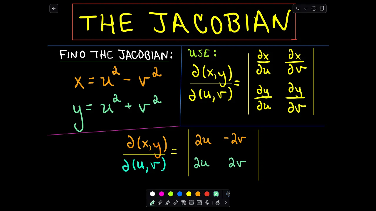



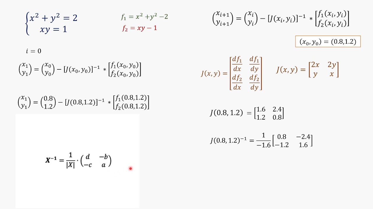

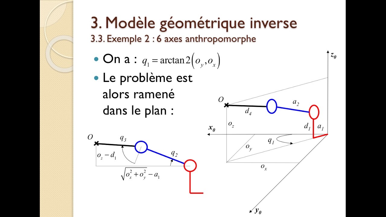

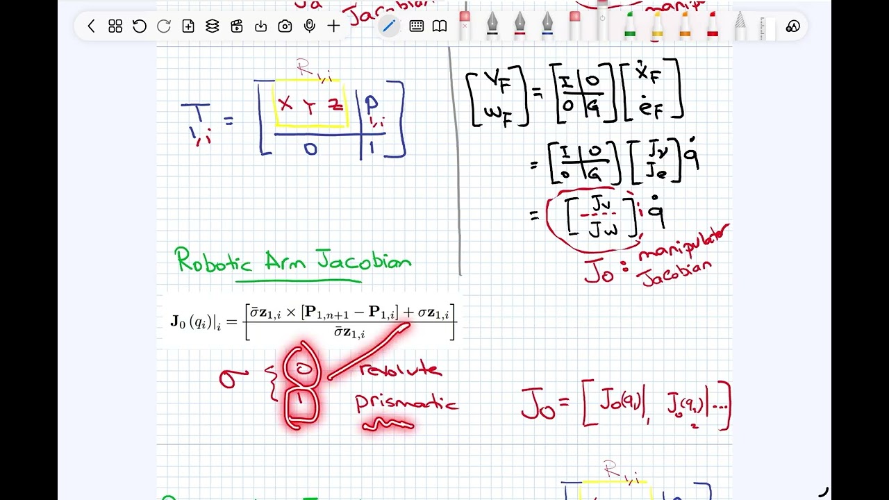


The Jacobian matrix is a 2x2 matrix that represents the linear transformation approximating a multivariable function locally near a specific point; it contains all the partial derivatives of the function's output components with respect to each input variable, where the first column shows how a tiny step in the x-direction transforms and the second column shows how a tiny step in the y-direction transforms, allowing us to understand the function's local behavior as a linear map.
Jacobian Matrix Explained | Local Linearity & Transformations
Added:Understanding of partial derivatives and the gradient vector in multivariable calculus.
Fundamentals of linear algebra, specifically how matrices represent linear transformations of vector spaces.
The concept of local linearity and tangent line approximations from single-variable calculus.
Familiarity with vector-valued functions that map input vectors to output vectors (functions from R^n to R^m).
Using the Jacobian determinant (the Jacobian) for change of variables in multiple integration.
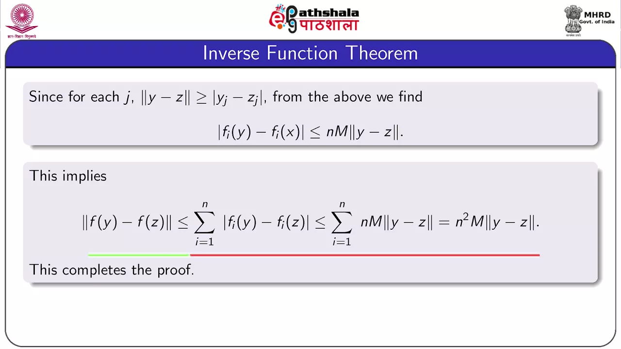
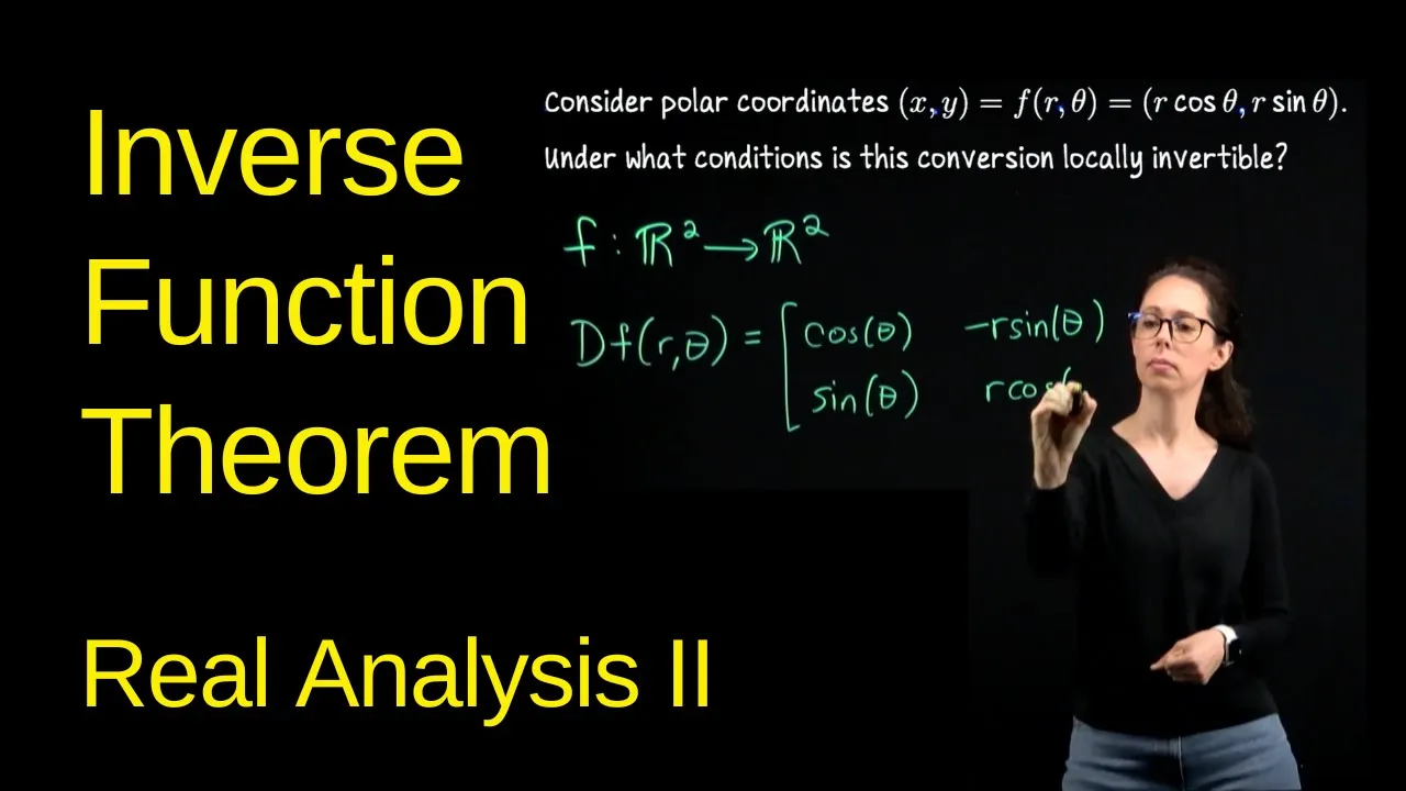
Applying the Inverse Function Theorem and Implicit Function Theorem in higher dimensions.
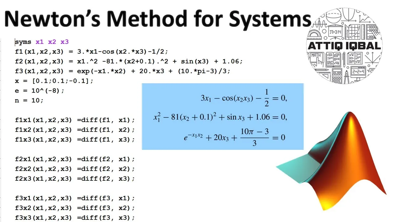
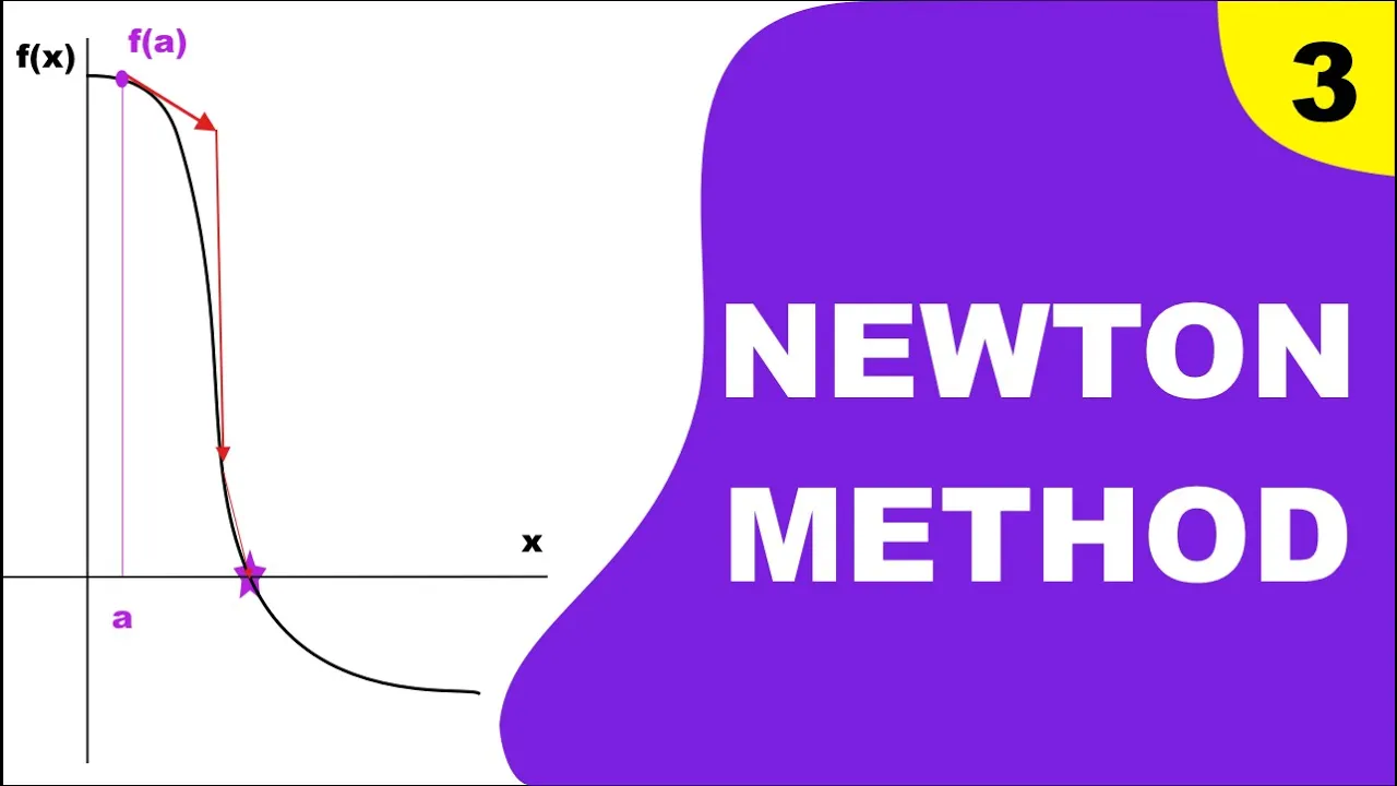
Implementing Newton's Method for solving systems of non-linear equations in numerical analysis.
Exploring robot kinematics, where the Jacobian matrix maps joint velocities to end-effector velocities in physical space.
580.9K views5.6Klikes6:22Original Release: 2017-01-10
in the last video we were looking at this particular function it's a very nonlinear function and we were picturing it as a transformation that takes every point x y in space to the point X+ sin y y + S of X and moreover we zoomed in on a specific point and let me actually write down what point we zoomed in on it was -21 that's something we're going to want to record here -2 one and I added a couple extra grid lines around it just so we can see in detail what the trans formation does to points that are in a neighborhood of that point and over here this Square shows the zoomed in version of that neighborhood and what we saw was that even though the function as a whole as a transformation looks rather complicated around that one point it looks like a linear function it's locally linear so what I'll show you here is what Matrix is going to tell you the linear function that this looks like and this is going to be some kind of 2x two Matrix I'll make a lot of room for ourselves here it'll be a 2x2 matrix and the way to think about it is to First go back to our original setup before the transformation and think of just a tiny step to the right what I'm going to think of as a little partial x a tiny step in the X Direction and what that turns into after the transformation is going to be some tiny step in the output space and here let me actually kind of draw on what that tiny step turned into it's no longer purely in the X Direction it has some rightward component but now also some downward component and to be able to represent this in a nice way what I'm going to do is instead of writing the entire function as something with a vector valued output I'm going to go ahead and represent this as uh two separate scalar valued functions I'm going to write the scalar valued functions FS1 of XY so I'm just giving a name to X Plus sin Y and FS2 of XY again all I'm doing is giving a name to the functions we already have written down is when I look at this Vector the consequence of taking a tiny DX step in the input space that corresponds to some 2D movement in the output space and the X component of that movement right if I was going to draw this out and say hey what's the X component of that movement that's something we think of as a little partial change in F1 the X component of our output and if we divide this if we take you know partial F1 divided by the size of that initial tiny change it basically scales it up to be a normal sized Vector not a tiny nudge but something that's more constant that doesn't shrink as we zoom in further and further and then similarly the change in the y direction right the vertical component of that step that was still caused by the DX right it's still caused by that initial step to the right that is going to be the tiny partial change in F2 the Y component of the output because here we're all just looking in the output space that was caused by a partial change in the X Direction and again I kind of like to think about this we're dividing by a tiny amount this partial F2 is really a tiny tiny nudge but by dividing by the size of the initial tiny nudge that caused it we're getting something that's basically a number something that doesn't shrink when we consider more and more zoomed in versions so that that's all what happens when we take a tiny step in the X Direction but another thing you could do another thing you can consider is a tiny step in the y direction right is we want to know hey if you take a single step some tiny unit upward what does that turn into after the transformation and what that looks like what that looks like is this Vector that still has some upward component but it also has a rightward component and now I'm going to write its components as the second column of the Matrix because as we know when you're representing a linear transformation with a matrix the First Column tells you where the first basis Vector goes and the second column shows where the second basis Vector goes if that feels unfamiliar either check out the refresher video or maybe go and look at some of the linear algebra content but to figure out the coordinates of this guy we do basically the same thing we say first of all the change in the X Direction here the X component of this nudge Vector that's going to be given as a partial change to F1 right to the X component of the output here we're looking in the output space so we're dealing with F1 F1 and F2 and we're asking what that change was that was caused by a tiny change in the Y y direction so the change in F1 caused by some tiny step in the y direction divided by the size of that tiny step and then the Y component of our output here the Y component of the step in the output space that was caused by the initial tiny step upward in the input space well that is the change of F2 second component of our output as caused by Dy as caused by that little partial Y and of course all of this is very specific to the point that we started at right we started at the point -21 so each of these partial derivatives is something that really we're saying don't take the function evaluate it at the point to1 and when you evaluate each one of these at the point 21 you'll get some number and that'll give you a very concrete 2x two Matrix that's going to represent the linear transformation that this guy looks like once you've zoomed in so this Matrix here that's full of all of the different partial derivatives has a very special name it's called as you may have guessed the Jacobian or more fully you'd call it the Jacobian matrix and one way to think about it is that it carries all of the partial differential information right it's taking into account both of these components of the output and both possible inputs and giving you kind of a grid of what all the partial derivatives are but as I hope you see it's much more than just a way of recording what all the partial derivatives are there's a reason for organizing it like this in particular and it really does come down to this idea of local linearity if you understand that the Jacobian matrix is fundamentally supposed to represent what a transformation looks like when you zoom in near a specific point almost everything else about it will start to fall in place and in the next video I'll go ahead and actually compute this just to show you what the process looks like and how the result we get kind of matches with the picture we're looking at see you then
Up Next
109:07
Calculus 3 Lecture 13.1: Multivariable Functions, Domains, and Level Curves
@ProfessorLeonard
767.2K views•2016-03-10

4:43
Elliptic Curve Cryptography Explained: ECC, ECDSA, ECDH
@PracticalNetworking
28.5K views•2024-10-21

8:12
Prime Numbers Explained: Definition & Examples | Pre-Algebra
@khanacademy
1.6M views•2011-05-12

6:00
The Mathematical Impossibility of Accurate World Maps
@Vox
23.3M views•2016-12-02
Related Study Plans & Knowledge Roadmaps
Structured learning paths in Mathematics
mathematics
Tensor Calculus: Vectors to Riemann Curvature
01Mathematical Foundations: Linear Algebra & Calculus
02Covectors, Dual Spaces, and Tensor Basics
03The Metric Tensor and Index Gymnastics
+ 2 more learning modules
40h5 modules
Explore Roadmap
mathematics
Gödel's Incompleteness: Logic, Proofs & Limits
01Introduction to Formal Systems & Hilbert's Dream
02Set Theory, Cardinality, and Cantor's Diagonal Argument
03Arithmetization and Gödel Numbering
+ 2 more learning modules
14h5 modules
Explore Roadmap
mathematics
Galois Theory: Fields, Groups & Solvability
01Foundations of Abstract Algebra: Groups & Fields
02Polynomials & Field Extensions
03Splitting Fields & Symmetries
+ 2 more learning modules
24h5 modules
Explore Roadmap
mathematics
Non-Euclidean Geometry: Models & Geodesics
01Euclid's Fifth Postulate and the Birth of New Geometries
02Hyperbolic Space and the Poincaré Disk Model
03Geodesics: Defining Straight Lines in Curved Spaces
+ 2 more learning modules
15h5 modules
Explore Roadmap