













![[LIVE RESPONSI UTS B24] Calculus - Function of Two of more variables](https://i.ytimg.com/vi/bECofN5w0aY/maxresdefault.jpg)







Multivariable functions require one more dimension than the number of independent variables to graph (2D for one variable, 3D for two variables, 4D for three variables), while their domains are graphed in the same dimension as the number of independent variables; to find the domain, apply the same rules as single-variable functions (denominators ≠ 0, square roots require non-negative radicands, ln requires positive arguments), and level curves are created by setting the function equal to a constant K and projecting the resulting curves onto the xy-plane to create contour plots that reveal surface behavior.
Calculus 3 Lecture 13.1: Multivariable Functions, Domains, and Level Curves
Added:A strong understanding of single-variable functions, specifically how to determine their domains, codomains, and ranges.
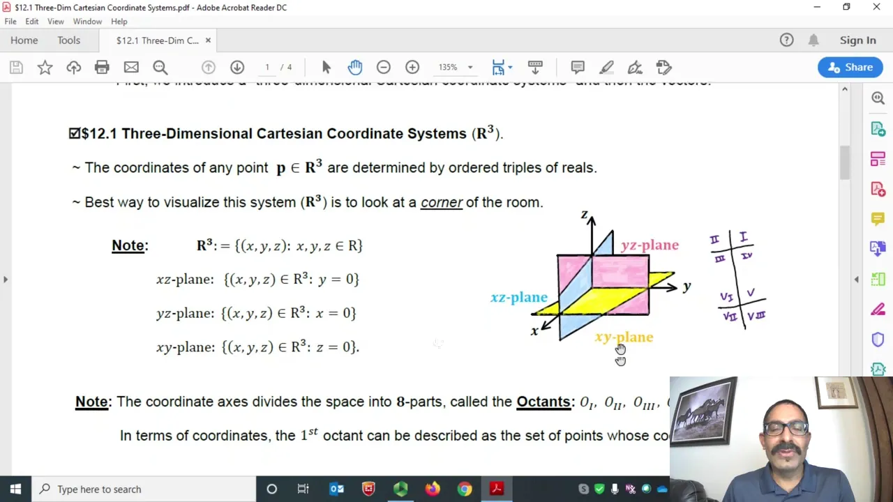
Familiarity with the three-dimensional Cartesian coordinate system (R³), including plotting coordinates and basic surfaces such as planes and spheres.
Knowledge of 2D curve sketching, particularly conic sections (circles, ellipses, parabolas, and hyperbolas), which are essential for analyzing and drawing level curves.
Basic algebraic skills for manipulating multi-variable equations and solving inequalities to find domain boundaries.
Evaluating limits and determining the continuity of multivariable functions using different path approaches.
Calculating partial derivatives to understand how a multivariable function changes with respect to one variable while holding others constant.
Exploring the gradient vector and directional derivatives, including the geometric property that the gradient is perpendicular to level curves.
Applying these concepts to multivariable optimization, such as finding local extrema, saddle points, and utilizing Lagrange multipliers for constrained optimization.
767.2K views11Klikes1:49:07Original Release: 2016-03-10
So uh new section, new chapter, some cool stuff. Uh we get to talk about finally some multivariable functions.
How these things work, how they look, and especially how the calculus relates to them. Because when you start dealing with more than one variable, what I mean by that is more than one independent variable, things get kind of screwy.
Like what's a derivative when you've got more than one independent variable?
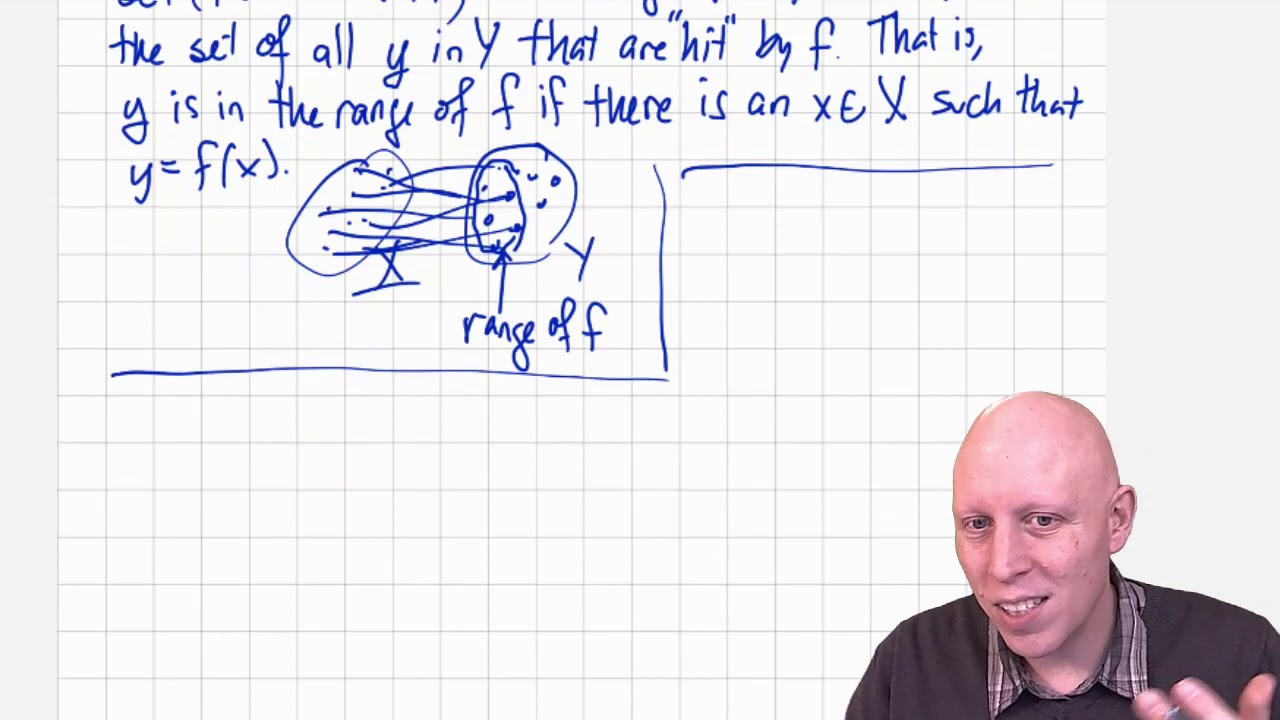
That's what we're trying to answer. and and we we start that with just an introduction about what these things do, what the domain is, and and how they work. So, we're used to talking about functions, but we're used to talking about functions in just one variable.
Please get this straight. When I say one variable, I mean one independent variable. So, like with X, the dependent variable Y, there's always only one dependent variable. All right? But now we're going to start saying, okay, uh, what happens when we have more than one independent variable? Well, there's good news and bad news. The good news is that the same stuff basically works. You still have a domain. You still have a range. You still get pretty pictures out of it. That that's the good news. The bad news is there's a little bit more aspects to it, especially when we start talking about like limits of more than one variable. That's the next section.
Okay, don't worry about it right now.
But what happens to these things? Um, here's here's some ideas. Here's some things that you need to know before we go any further. So, number one, in order to graph a function, these are universal. In order to graph a function, you have to have one more dimension than you have independent variables. We're always going to revert back to independent variables. We talk about those things. You always have to have one more dimension than you have independent variables.
By the way, the reason that we talk about independent variables and not total variables is because when we do function notation, The only thing you really can count really easily is independent variables. That's why we talk about Let me give you some examples here real quick. So, how about how about that one? Very simple stuff, but how about that one? Um, how many independent variables do we have here? One independent variable. What is that independent variable? By the way, you can always do this no matter what.
We can always go from function notation to dependent variable. So there's one independent variable, there's one dependent variable. What how many dimensions would you need to graph this graph? Two.
Notice it's one more dimension than the number of independent variables you have. So we have a direction for the x.
We got a direction for the y. That's that's two d that's two dimensions. Two directions. So this would be graphed in 2D.
Now we step it up. A function with two variables listed like this. By the way, whenever you see your function notation, we have another one in a second. This always lists out for you always what your independent variables are, no matter what. So here we got one independent variable. It's only X. Here we got two independent variables. They're X and Y. We're going to talk a lot about what that means. In order to get an output, you no longer need just one number. You have to have two numbers. You literally have to have a point on the xy plane. And when you plug in that point, it gives you out a height. So given a point xy on the xy plane, you plug it in, you get a height out. That's why we have the 3D coordinate system laid out the way we do where it's flat surface where you plug in points and at every point this function gives you a height. If you take at every point you find a different height, it's going to give you this surface. Well, let let's think about that. If we have two independent variables, verify two independent variables, a function based on those two independent variables. In order to do this, in order to take those two independent variables and be like, okay, on my xy plane that's flat and take a take a point out here somewhere and I plug in that point, two values, two numbers, and I get this height. I get a different height at every single point. It's going to create this surface in what dimension? Two independent. What dimension do I need to graph it in? 3D. I need 3D to graph not only the X and Y motion, those points, but also the height above it. So that's a 3D a 3D necessible. We need 3D to graph that surface. Also, you can always do this just go one variable different than what you have for a dependent variable.
If we have g of xy = x^2 + y^2, we can represent that z = x^2 + y^2. Um, I'd like you to get used to to knowing these things mean the same thing. You you know it from a long time ago that f ofx we can replace with y. But now any function we can replace with one dependent variable. Notice if we follow this you will have at most how many dependent variables?
One one dependent variable because we have these functions based on independent things. We say hey let it equal a variable. You can only do that one time. There's only at most one dependent variable. Head on if you're okay with the idea so far. Let's step it up one more time. This is be kind of cool kind of crazy.
So first thing recognize the function notation. Hey uh ladies and gentlemen left hand side how many independent independent variables do we have? Three.
Can you tell me what the independent variables are?
This always gives you the independent variables every single time. So this one said just x. Hey, there's only the x's.
This said x and y. Hey, there's x and y.
This says xyz. There's three independent variables. Could I write it not in function notation but base it on? Well, how many dependent variables could we maximally have? How many? One. So the dependent variable, call it something like w not x, y, or z. Says the same thing. Now this is weird. All right, let let's picture this for a second. Picture what this is this is going to be. I know you can't see what the graph is. That's okay. Neither can I. But but I want you to think about what's going on with this. Just just track with me here for a second. If I plug in one number, that one number is on the x axis. Correct. I'm going to get a height. That's what the y is. So I go over. Okay. So that's one dimension, two dimension. That's all that's happening.
If I plug in two numbers, I'm plugging in an ordered pair. That's a point on the xy plane. That's why we have x and y. It's on the xy plane. I plug in that point. I use it in a function. I'm going to be getting out a height. So at every point I get a height. That's the 2D combined with a height. That would be three dimensions. That's why two independent variables gives you three dimensions. What would three independent variables give you?
Four dimensions. Four dimensions. What?
Think about it. This this is an order triple. It means you give me an x, a y, and a z. You plug it in, you get something else, you get a fourth dimension. How we graph it? I don't know. It's really hard to think in 4D. How do we represent 4D? We live in a 3D world. What would that 4D be? Some people use time to represent the changing of the 3D system over time as that that fourth dimension. Um, but it's you can't draw it. You can't draw it. We need one dimension lower to draw.
Well, you can, but it's got to be able to move. Uh, you need one dimension lower than the graph to be able to represent it. For instance, you can represent 3D on a plane. Uh, but 4D, you need a 3D model to do that. You need to draw it on 3D. So, do you see the do you see the point though? No pun intended, but do you see the point? If I give you an ordered triple and plug it in, it's going to give me something greater than that, some dimension more. So for one independent variable we need 2D to graph it. For two independent variables we need three. We need one more dimension. Then however many independent variables we have and this is like I'm sorry. Okay.
Or what uh yeah 40 is weird to think about what we typically do for graphing.
Well you know we'll get to it later.
We'll get to it when we actually start graphing these things. Right now I want to know if you understand the concept of one independent variable two dimensional picture two independent variables threedimensional picture that's what I want know if you understand the concept that the the two independent variables is the point height above the point gives you something in 3D this surface now let's talk about the domain because the domain we spent a lot of time talking about domain here to graph the domain Hey. To graph the domain of the function, you've got to have a dimension equal to the number of independent variables. It's one lower than the graph itself. So, well, we'll talk about in a second, but write write this out. To graph the domain, you have to have the same dimension as the number of independent variables. We always revert back to independent variables.
So let's see. Let's see. Everyone in class right now, you should be at this point. How many independent var you How many independent variables do I have right here? How many independent variables do I have right here? How about here? So if we're graphing the domain, we're literally graphing the that variable. Well, how many dimensions do you need to represent numbers on an x-axis?
One. One. You just need the x- axis. So, in order to graph the domain of a function, just the domain, we need the the dimension equal to the number of variables. Here, for the domain, we need just one d, just the x-axis. That's it.
How about this one? What if you wanted to math? This should man, this should make a lot of sense. Okay. How many dimensions do we need to graph the domain with two independent variables?
2D. Well, think about why. If the domain, look, if the domain are XY points, do you guys get it? We plug in the point, we get a height. If the domain is the XY XY points, we need something on the XY plane to graph those points. The domain here would be in 2D, just something on XY. This is a weird one.
What if we had a function with three independent variables? We talked about that. It's got an x, it's got a y, it's got a z.
It's in three space. What do I need to describe that domain in is I need 3D. I need to be able to represent x, y, and z. So that's why we have this this this statement here. If you have one independent variable, you need one dimension to describe the domain.
Two independent variables, two dimensions. Three independent variables, three dimensions. Please don't get these two ideas confused. The picture is always one dimension more because you're plugging in two things and getting out the third. Plug in three things getting out the fourth. But to graph the domain, we have the equal number of dimensions for that. Uh this will become a lot clearer when we do some examples. But right now, do you understand the concept behind it of the number of independent variables, what the graph looks like, whether it's higher and what the domain looks like, equal number dimensions.
Show hands feel okay with that idea?
Okay. Are you sure? Any comments, questions or anything before we continue? Yeah. If we had four uh independent variables, would we not be able to graph it at all? Graph the function or graph the domain? Uh the domain the domain would have to be graphed in 4D with four independent variables. You'd graph in the domain in 4D. The shape would the the surface it's called a surface. The surface would be graphed in 5D. 5D.
Sure. Go for it.
Uh let's try let's try just practice.
Let's just practice one just to get a a feel for the taste of how these things work.
So we're going to talk about domain in just a second. I want to see if we can just look at a function and do some stuff with it that we normally do like plug in a point, manipulate the stuff.
What can we do?
And I want to make sure you were paying attention, ladies and gentlemen. Firstly, function.
Yes. No. What do you think? How many independent variables do we have? How many dependent variables would we have?
How many total variables do we have?
Four. Four. How many dimensions do we need to graph this shape? Four. four one more than the number independent because you count the dependent. So total number of variables total dimensions for the shape number of independent variables got have one more than that for the shape. So this would be a 4D graph. Next question. Right side only.
How many dimensions do you need to graph the domain of this thing?
So, we need 4D for the shape, whatever the surface is. We need 3D for the domain or something called a contour plot. Uh, we haven't talked about contour plots yet, but we will. I'll show you exactly how they work. They're not too hard. Uh, do you remember traces from section 11.6? Those are pretty much what contour plots are.
Uh so we take those and project them and then we get this contour plot. Have you ever heard of topographical maps? Yes, that literally is a contour plot. That's what that is. It's taking different It's what what's doing is taking this mountain range, right? And going up 100 feet and 100 feet and 100 or some segment that's always the same and saying, "Hey, make a make a a curve that's level around that surface and then look down as you like on a as you're projecting to a plane." And that's what a contour map is. So we talk a lot more about that how to find it.
Could you do stuff like if I asked you find the function evaluated at 021? Could you do it? Uh what would you plug in for the x and the y and the z1? Yep. The order triples. Notice how it's in order triple has to be in 3D.
That's why the domain is 3D. If we plug that in, we get well, let's see. 0 2 + 2 * 2 2 3 * -1 2 = 11<unk> 11. Notice what you're doing. You just took something that has a 3D representation in order triple. You plugged into a function. It gave you a different number out. It gave you something that depends on what you plug in. Your dependent variable value would be that height in 4D over that point in 3D. That's what's going on here. Are you sure you're okay? For real. We can also do one more thing with these just for right now before we start talking about domain. I'm just making this up. Uh, that's coming out of nowhere. I'm just making up this representation. But, but check this out. If you had a way to parameterize X, Y, and Z in terms of another parameter like I don't know t remember that like another parameter.
Sometimes we can we can trick the problem a little bit. We say, hey, can I change all of these into values of u and make it a little bit simpler to at least work with? Yeah, sometimes we can. So if we have this parameterization, what would you plug in for X? What would you plug in left side for Y?
And what would you plug in for Z?
Why don't you try that right now? Try it. Distribute it. Simplify it. See what you get. I'm going to do on the board as you're doing it. I'll do a step about every 10 seconds or so. See if you can substitute this in and change this into terms of u.
Hopefully that's not the screen. I don't know. It was pretty close.
So just a a quick and simple manipulation we're able to get at least the first part substituting that in that composition should be okay with the idea of just what what these things are. So a little just a little 20 second recap. Uh we got these things called multivariable functions. Now with one independent variable takes 2D. Two independent variables 3D. Total number of variables equals what you need to graph it. 2 3 3 4. It's always one more than the number of independent. Domain it's always equal to the number independent. That makes sense. You got one you one dimension.
Two you got to have two dimensions.
three, you got to have three dimensions.
You got to have that our coordinate system. So, what we're going to focus on right now is finding domain. As I, man, as I mentioned to you, um, finding domain is huge as far as your ability to to graph a region to integrate over.
When we get to chapter 14, we're going to be integrating over these things. Um, and and understanding what we're actually doing. What region are we integrating over? That's important.
That's what we use this domain for. I'll show you exactly how to do it when we get there, but it all starts right here.
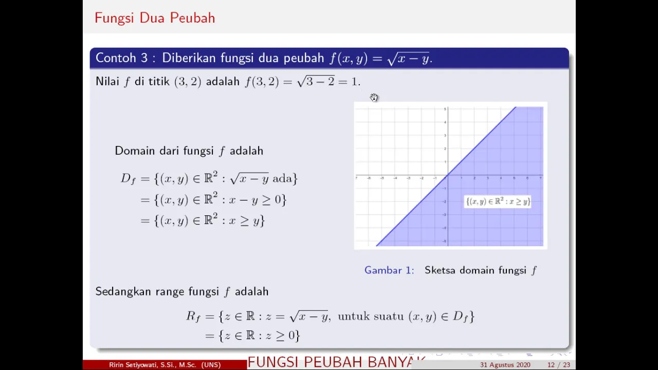
So let's do some domain. Let's see exactly how it works. I'll show you some uh some things you can do, some things you can't do, and some things you absolutely must do. So first one, I'm also going to really focus on your ability to understand what dimension we're working with. So we're going to do a couple things. We're going to find domain and we're going to find range. Here's the cool stuff. Uh the same things you're you're looking for like for domain of any one one variable function, one independent variable function. Same stuff you look for here, which are like square roots, natural logs, anything that has the possibility of being undefined. It's the same thing you look for. So denominators, they should be slapping you in the face. Uh those sort of things, they work universally for functions and we're going to use them here. Um so when we look at that one ladies and gentlemen function yes no everybody how many independent variables do we have how many total this would be graphed the surface itself would be graphed in and the domain would be graphed in I'm going to show you how to graph domain in the next few section sorry uh examples right now I just want to get a feel for what the domain is so let's take a look at it does the numerator give us some things that have a possibility of not being defined If I multiply any two numbers, even if I get zero, I'm good to go. Not a problem.
How about the denominators? What do you know about denominators? Like universally any fraction, what do you know about them? So, what we know is that x - y in no way can we ever let that equals zero. Does that make sense?
Yeah. Okay. Um, solve it. Just solve it.
Okay. Well, if I solve that, then what that means is that x can never equal y.
As long as we don't have x equaling y, we're good. We can plug in anything. Do you do you recognize that from I gave you the easy one to start with, but you recognize that? As long as these two numbers aren't the same, we're fine.
That's exactly what this says. Now, all we've got to do is put that in domain.
Now, it looks a little strange, uh, but it's the same statement as having one independent variable. go. Okay. Well, the domain would be a set of numbers. We use set notation generally. It's pretty hard. Well, it's not super, but it is difficult to describe it other than this because this is well, this is the nicest way I know of that we can go, well, what's what what's our what's our inputs? What is our independent variables? What are our independent variables here? XY. So, every time we plug something in, it's an ordered pair.
So the domain says hey you've got ordered pairs x y what can you h what can you let happen so such that what can you let happen I can let anything happen any ordered pair the only exception I have right now is that x cannot equal y that right there is the domain in English it says it says this it says the stuff you can plug in are any ordered pairs but not such that x does not equal y or but x can't equal y. That that's all there is to it. Should be okay with that one. Now, the range still works the exact same way as it always does, but you're going to call it the output. So, if we have inputs x and y, what traditionally do we call the output variable? Z. Okay. So, range works the same way. But for range, uh range call the out. Oh, sorry. Range will be the output. Call it Z. So for the range, a lot of people struggle with the range. It it sometimes requires a lot of thinking like what what could we possibly have?
So is it true that we can get anything out of this? And the answer is yeah, it's it is true. You can plug in a lot of difference. As long as x doesn't equal y, we can get infinity. We can go down to negative infinity. We can get zero. Uh no problem. Just let x equals 0 when not y is not zero and you get z.
Yeah, you get zero. Um so 0 * y over 0 minus something not zero, you'd get zero. So we can get the whole spectrum of outputs here. And how we represent that? How do you represent that? What would you do?
How do you represent Z? The range can be anything.
Yeah, the same thing here. So Z such that Z is between these two infinities. Just make a little side note just in your head.
Just in your head, how many how many independent variables do you have?
The domain has to say something about all of them. So your domain must include all the independent variables. Got to make a statement about all of them. The range should have only how many? One.
One. Just the dependent. So domain's got to say everything about all these variables. Got to have a statement about that. The range would include just your one dependent variable. Show hands feel okay with that one. I know I'm talking it over a lot, but honestly, when we when you guys first see functions, you're in a class mixed with a lot of other people who aren't going on in math. And so, sometimes it's not taught very well. I know that I kind of skim through it myself when I'm teaching to people who aren't going into calculus.
Uh, but you need to be familiar with it, which is why we're taking a little bit of time here to make sure you actually understand what it is that we're doing.
Does that make sense? We're going to do especially that when we get to graphing.
Let's try one more just talking about domain and range. Then we'll start graphing the domain. Then we'll graph the range which is a surface. So as I mentioned man, you get you get the same sort of problems with um with functions with two variables that you have with one variable. So we look for things like square roots. We look for denominators. We look for ln.
We we look for those things that have possibilities of not being defined. So when we look at this uh first thing everybody, how many independent variables do we have? How many dependent variables do we have? What would you call that dependent variable? In what dimension would you graph the surface here? One, two, or three? In what dimension would you graph the domain?
Perfect. So let's talk about the domain.
Uh which side I uh go right side. Give you guys a chance. Tell me something about what you know about this function.
What do you know? Can't be negative.
What can't be negative? The output.
Okay, the negative the output can't be negative. I know that. Tell me something about the domain. What about the inputs?
What do you know about square roots?
More specifically, what do you know about the inside of square roots?
They can't be. So, use that, man. Use the one thing you know. What we know here is that the the radicand the inside of our our radical here for square roots has to be greater than zero question. Can it be equal to zero?
What if it was on a denominator?
Okay. So, so use that. So, this can be equal to zero since I don't have this on the bottom of a fraction. We're fine.
and know if you're okay with that one.
Now, all you got to do, I promise this is it. All you got to do, solve it for x and y. Solve it so that you have some expression here. This this is you're literally done. Okay, this is it. All we got to do is make sure that we have x and y. Okay. Well, let's let's add these. Done. Practically practically done. Practically done.
head if you're okay with how to get that. Yeah. So, what I know is that any ordered pair, any two numbers when I square them and add them, they have to be less than four. There's not a better way to say that. We I we can't say that a better way. Putting this in terms of y less than well, we have minuses and pluses there, but also we we have this.
Can you ever get this to be a negative?
No. So, we also know this is greater than equal to zero. x^2 + y^2 is always positive. You cannot add two numbers after squaring them and having them be negative. That's what our domain is. So our domain says okay I have a set of ordered pairs where my coordinates are x and y and I need these ordered pairs to do this. I need them to be bigger than zero. That's not right. But I also need them to be less than four. Yeah. So, would it be incorrect if you forgot to put the zero? No. I think that's how I first had it. I'm just going to use this for the next step. So, if you have this, that's that's sure.
That's correct, too.
I'm just going to use that zero thing for the next part. So, that's a good question. Any other questions? Do you guys feel okay with how how to get that? Now, some of you guys are looking at me like, okay, let's let's go through one more time. Do you understand that square roots can't have negatives inside of them? Yes, that's what that says.
That just solve for some expression that relates x and y to some numbers. Here, it was pretty easy because we we could solve for a variable. Here it's not that easy because when I start solving for variables like that firstly I lose the picture of the circle cylinder that we're going to get. So it's really nice to keep them in terms of things that we know we can actually graph in hey 2D. What dimension would it take to graph this 2D? It would take two independent variables 2D. You can graph that in 2D. That's not hard to graph in two dimensions. It's a circle radius of four and everything included including that. That's that's all I'm asking you.
When we start trying to solve for y, we start losing that. You start getting pluses and minuses because you got that square root in there. Do you guys see what I'm talking about? That's that's nasty. So, we just relate these variables to your number. And that that's all I'm asking for. Now, let's talk about the range. Are you better at this? You okay with that? Let's talk about the range. What variable would you use for the range?
This takes some thought. You got to really think what can you get out of this? What can you get out of this thing? What's the maximum? What's the maximum this could be given this scenario? What's the maximum this could be? Well, the maximum this could be is because this has to be positive. Verify that that x^2 + y^2's got to be greater than equal to zero. You can't add two numbers together that have been squared and get a negative. It's not possible. So the small the largest this can be and smallest this can be is going to be based on the fact that the largest this can be is four. But the smallest that can be is zero. What that means is that if we if we add these two together and get four, if you don't see it, I'll do this. Might be easier for some of you to see. Factor the negative. If we add these together and get four here, what's the smallest this could possibly be?
Zero. So, our minimum for our range is zero.
What's the maximum that this could be?
Notice notice uh the maximum this could be the smallest this can get is zero.
So, if the smallest this can hit is zero, what's the maximum this range could be? out could be not four. What is it? Two cuz it did you did you follow that? Most of you did. Some of you didn't.
Um I can only let this get and this is why I wanted it with a zero. Okay. This is this is why if you let that happen, check it out. This number has to be between 0 and four. You get it? Which means that if I plug in zero, I'm getting out of four two. If I plug in four, I'm getting out zero. So the the range here, the range of outputs is 0 to two. Not 0 to four, square<unk> of four. Some of you guys are just writing down stuff and you have questions. What questions? Come on. I know there's got to be something out there. Do you understand why it's two and not four? Do you understand why it's not more than four or more than two? Do you understand that?
What's the lowest? Did you guys get this? That factor in the negative. The lowest this can be is zero. It can't get smaller than that.
4 - 0 is 4. Square of 4 is 2. The biggest this can be is four. If it's more than four, we get something undivided. We get imaginary numbers. We don't let that happen. So, the most that can be is four. 4 - 4 is zero. We're somewhere between zero and two. That's it. That's all we're That's all we're doing. It's all we're about for real. Show hands feel okay with the idea. We're going to move on. We're going to start graphing these things.
I'm going to start really slow uh with graphing regular old domain like from one one independent variable functions.
We'll do one of those and then we'll start stepping it up a little bit. We'll end up getting to how you graph domain with three independent variables.
By the way, don't blow off the section even though it's boring and you don't like graphing because graphing the domain here let you solve double integrals and triple integrals later.
It's it's important for you if you've had this class before. I know there's some of you you know that what I'm saying is true because you go, "Oh, how do you find the region of integration?" Uh you you you graph it.
You go, "Oh, crap. Shoot. I forgot I forgot to graph anything." Oh, this is going to be fun next semester for you.
Just kidding. Just kidding.
Oops. Did that come out?
See you next year. Oh, okay.
Yeah. Just remember this. To graph the domain. What? How? What do? Okay. So, if you have one independent variable, how many dimensions for the domain? Two independent variables.
You need a axis for each independent variable. You need a domain or sorry a a dimension for each independent variable.
So to graph domain To graph domain, you have to have an axis for each independent variable. This will work all the time for your domain. Okay, quickly everybody quickly.
How many independent variables do we have? What is that independent variable?
You need one axis. You need the x- axis.
That's enough to graph the domain. So for our domain, you go, okay, what do you mean? How how can I graph that?
Look, here's the here's the x axis. If you let this, you know this x has to be greater than zero. Correct?
Can't be equal to zero, but the square root is going to be greater than zero.
Must be strictly greater than zero. Can you graph that on just the x-axis?
Here's zero. Here's this way. You have parenthesis saying I can't include zero and it's everything positive in that.
That's that's a simple number line. Oh my gosh. Yeah, you're right. You can graph domain on just a number line if you have one independent variable.
That's literally all that we are doing.
Sure. Feel okay with with that one. Now, that's basic domain. You should have learned a long time ago, but we run with that. We we do the same thing here. So, let's try this one.
Everyone right now. Everyone right now.
How many independent variables do you have? That was supposed to come out. How many independent variables do you got?
Sounds like I'm drunk sling words up here or something. My bad. How many do you have? Two. Okay. What specifically do you have?
So, we're going to need two axes. What axes. To graph the domain with two independent variables, you got to have two axes. So, first thing we're going to do, just like we stated domain here, we're going to state the domain here. Same stuff we did. We're just now going one more step. We're just going to be graphing this now. So, can we figure out what needs to happen with this thing? Uh, well, it has no square roots, but it's got denominators. What do you know about denominators?
can't be zero. So I know x^2 - y^2 cannot equal z for sure. Yeah, it's a denominator. Can you solve this for one of the variables? No. How do you know what to do when? Well, if you have zero, there's not a constant, then it's not giving you a picture that's very nice.
It's not giving you a hyperola. It's not giving you a circle. It's not giving you an ellipse. It's giving you, oh, I could probably just solve this for y if I wanted to. If I solve this for y, I get y^2 can't equal x^2. Does that make sense? Let's go a step further. Can you literally solve it for y? You see the idea of trying to get something we can actually graph that you recognize that you can graph it. You should recognize that you can graph that as a circle.
Actually, it's a it's a dis. It's it's the inside of a circle. Do you see it?
It's a whole bunch of circles put together. It's the inside of the circle from the origin out to a radius of two. That's all we're doing. Well, let's figure this one out cuz y^2= x^2 doesn't look so hot to me. Uh, but if I take a square root on both sides, and you need to know this, when you take a square root, it's not on your paper, but then you put it on your paper, what must you have all the time?
So, y cannot equal plus or minus x.
use that. I want a set of points XY such that Y can't equal X and Y cannot equalX. Here's the question to you. Don't overthink it. Don't overthink it. Can you graph y= x quickly? What's the uh y intercept?
What's the slope?
Can you graph y equals negativex? What's the what's the intercept? What's the slope? They're two diagonal lines like that. That's all that's all there is to it. So, since we have two independent variables, you need two axes. You just need the x and the y axis. Not that hard. You just need whatever independent variable you got, put an axis there. You need the x and the y. If we graph y = x and y=x. Now, now you do have to understand what we're doing. Okay? So, if you if you didn't pick it up the first time, here's what we're doing.
Here's what we're doing. We're we're saying this. Can I can draw it and then look up here so I know you're done so I can talk at you.
Okay? Go ahead. Make sure you you get it down.
I don't want to talk over your writing because then you're going to miss two things. Here's the deal. What I'm saying here, what we're saying, what this is saying is I can take any point, any point on the plane, any ordered pair.
Ordered pairs are on the plane. They're on the xy. That's what we're talking about. Any point on the plane, provided these things don't happen. Provided I can't have y equal x. Do you understand what I'm talking about? Just can't be on that line.
Provided y can't equal negativex. I can have anything but that.
So what we're talking about here for the domain is literally the entire plane.
Literally the entire floor, the entire xy plane besides these two diagonal lines. So we're going to shade everything but that.
like 5second recap if you will. Every single time we're graphing domain, you need the number of axes equal to and the same axes as your number of independent variables. One x one x axis x and y x y axis xyz xyz axis. Uh in order to graph it, we solve domain like normal, man.
Just just the problems that are slap you in the face. Denominators can't be zero.
Great. Solve for it. Graph the lines, graph the circles, graph whatever you have and then shade the pieces that actually work here. So, this says any point works unless you're on the line.
That's why they're dotted. It says the dotted lines, you cannot be there. Any other point? Fine. Your answer okay with that one for real. Yes. No, you guys over here. You guys over here. Yeah. We got a couple. We got one more to do uh with this these two independent variables. Then we're going to step it up a little bit.
Do you guys take notes when I say test question? Do you take notes of that?
This one might you know That looks nasty, but man, don't don't overthink it. It's just talking about domain. You know what has to happen with your functions. You are familiar enough with with these things. They're not going to get any crazy new functions that happen. There's just some certain rules we can't break. We can't let denominators equal zero. We can't put negatives inside of even powered radicals. Uh we can't go negative with ln. We we can't even go to zero with with ln. You can't do those those things. If you mind the rules, just write it out. You're going to be fine.
Let's be real careful about this. So, first thing, uh, what dimension would you need to graph this surface? What dimension for the whole surface? What is it? How about the domain? What dimension? Is it pretty clear right now just looking at it? Oh, two variables.
Domain's got to be graphed on xy plane.
It's the floor. All right. Put it on the up here, but it's the floor. So, we're going to graph this on an xy plane. I'll just put it right here. Our goal is to get a good picture for the domain there.
Now, let's start working with it. What do you know? What do you know about ln?
I kind of ruined the suspense, if you will, but uh what do you know about ln zero? Strictly strict the argument of the natural logarithm has got to be greater than zero. Uh the ln looks like this for you guys. So, there's a there's this asmtote right at the the along the y- axis. You can't even get to x equals z. So, we're going to go the inside the argument can't equal sorry um has got to be strictly greater than zero. Don't put not equal. All right.
You you got to show me some inequalities if these things involve inequalities.
So, we don't say, "Oh, it can't equal zero." Yeah, you're right. But it's also got to be can't equal negatives. So, if you just put doesn't equal zero, that implies you could plug in negatives.
Does that make sense? Got to show inequalities if they apply. Could you solve that?
solve it for a variable that allows you to graph it. So if we have y - x= 0, that's not so much fun to graph. I don't know how to graph that very well. I can't do cover up method or anything as you learn in math C section 9.4 I believe. Math C. If you're not good at graphing inequalities, watch chapter 93, 94, I don't know. Math C intermediate algebra chapter 9 shows you how to graph inequalities pretty easily, pretty well. Um, so you can watch it, brush up on it. We're going to graph that in just a second, but that's only part one. That's this little one here. Are there any other pieces that are going to allow me to have some possible undefinedness? Square and tell me left center, just you guys over there. What has to happen with that particular radic? What do you know?
Is that it? Is that it?
Come on. Don't look at me with those blank eyes. Tell me. I don't know. It's dead eyes out there.
Goodness. I'll get you some more candy.
Not right now. It made a crinkling noise on last video. Pissed me off. So, no.
You got to get it during your break.
So, it's gross. All right. But I don't want to hear you chew. It's nasty. No one wants to hear someone chew. You ever heard someone Don't hearing someone chew and swallow is probably the worst sound. It's not as bad as a fart in church, but it's close. All right. You can't move. You're sitting there the whole time. Little kids. Whatever. Um, this is not it because I know, yeah, I know it can't equal zero, but also we know that square roots have to have positive radicans. That's another inequality.
Now, can you solve for that inequality?
Could you solve that for for y?
Do it. If you put just not equals all the time, you're going to not equal the right answer. I don't want that. I want you to get the actual inequalities involved with these domains. In this case, instead of subtracting subtracting, I'd probably just add and flip. So, we get y is less than x + one.
Hey now, if you're okay with that, now can you graph them? Recall that graphing inequality says graph the line and then shade a half plane above or below. If you have it y equals, it's really easy cuz if we graph this, if we graph this thing, by the way, should I graph this with a solid line or a dotted line? What do you think? Why? If we had the equals, we would have a solid line. This is the graph y equals x.
That's y equals x right there or not equal to x. That's what that is. Now, what this says is I want to shade. If you have this y equals all or y and then inequality all the time, you can always just shade above or below the line. It's pretty nice. So, this sh says I want to shade above that line. I want to shade the half plane. Now, don't do it now.
Don't do it now. Just keep it in your insa. Okay? Just keep it right in your head that you're going to you're going to shade above that line with me. Let's graph the other one. This one has a y intercept of one. It's got a slope of one. Same slope. They're parallel. Explain to me why I'm graphing this with a dotted line again.
Again, if I have this y and then inequality, it'll tell you whether to shade above or below. This one says shade y less than that. Shade less than that, below that. Does that make sense to you? Are you sure? Can you graph just y= x? That's all we're doing. Can you graph y= x + 1? Then put them together.
The inequalities say you're going to shade a half plane, but we also want both of these things to happen. We got to satisfy both of them. We need this to happen and we need this to happen. We need the the overlap. So, if I'm doing this, this is graph the line, got it, dotted line, no equals. Graph the line, got it, dotted line, no equals. But I need these half planes. This is above this one, but also below this one.
Can you see the region? It's a strip of points. That's all that's happening. So this our domain is every ordered pair in that strip in that segment. That's the best way we can graph our domain right there.
Um this really when we write our domain out and say okay well the domain is every ordered pair such that y is greater than x and y is less than x + 1. That's great. That's technically the domain.
But it doesn't give us a good picture of what's going on. This is a good picture of what's going on. Shows you literally shows you every single point of what we can. Now what are we doing? Is this the graph of that thing? No. No. But this is really interesting. This is the graph of the points. You could I hope that you're paying attention cuz this I I'm trying to teach you like four things at once.
All right. Uh what the graphs look like, how we're going to do double integrals later on. We're going to do all about all this stuff. If that's the domain, that's the strip of points I can plug in. Okay. Now, now picture this axis flat, the x and the y. Can you picture it? That's the strip of points doing this. That surface is just going, this is just the domain, just the crap we can plug in. The surface is going to be that whatever it is, whatever shape it is, but it's only going to be above that region. Do you guys get that? It's just above the region that I I just drew.
It's going to be this weird surface strip that's going through space. It's kind of cool. That's what's going on.
That's what I need you guys to understand. Why is it important to graph domain? because in doing so we can bet better understand how the surface is behaving where it's going to be over. If we know where it's going to be over, integration becomes easier. That's one of the major points here. Understand the concept. When we come back from a break, we're going to talk about how to graph domain with three independent variables.
Uh we'll graph just a couple of them.
Then we'll talk about um how to graph functions themselves. We'll do that.
We'll talk about level curves. All good.
So working with domain of these multivariable functions with more than two more than two independent variables.
Verify more than two. How many? More than three. We can still do the same thing. We still look for exactly the same problems. Um it's it's just this.
How many dimensions do we need to graph this surface? The whole thing. Four.
Yeah. Three independent. That's one dependent. Four variables. four dimensions or one more than independent.
To graph the domain, we'll need three.
So, we'll need three. We'll talk about what it is. I'm not going to specifically graph it, but the shape will be readily identifiable. What do you know about that function? Come on, quickly. What do you know about or at least the domain? What do you know about the the domain? What do you know?
So, the inside of this square root and if it helps you right away uh to to do this to go, oh, well, factor the negative You can go ahead and do that question.
Should I remove that equals? We did sometimes before. Should I remove that?
No. No. It's not a denominator. So, all I need is for this inside part to be positive. Show hands if feel okay with with that one. Now, let's group our x, y, and z's on one side. And let this is typically how we do it for 3D. Do you remember 3D graphing at all? Do you remember section 11.6? remember surfaces and all this stuff. Try to get one of those. So, if we group all of our x's and y's and z's, basically add this, we get x^2 + y^2 + z^2 is less than or equal to 9. So, be okay with that. You've literally just found your domain. That that's all there is to it. All I know is that these three the the combination of the squares of these sum of the squares of this ordered triple has to be greater than or equal to 9. I also know this if you take three numbers any ordered triple and you square them and add them will it be positive? The least it could be would be zero. So it's greater than equal zero.
Now please don't misconstrue this. Um I had a question during the during the break. It was a good question. Well, wait a minute. Can't you plug in a negative for x? Yes, you can. And you can plug in a negative for y and z. I'm not saying anything that this is individually each of those is greater than zero. That's not what I'm saying.
What I'm saying is that when you take a point and you square those values and add them, the combination of of the square, the sum of the squares of that point has to be greater than zero and less than nine. That's what I'm saying.
Does that make sense to you? That's what I'm saying. Not that each individual one. Yeah, you can plug in negatives here. No problem. But altogether when you plug it in and square them, it won't be it won't be negative and it can't be more than nine. So that right there, that's our domain. It's an ordered triple such that and you don't specifically need that. I'm just trying to tell you what it is. Uh such that that ordered triple sorry such that uh x2 + y square has got to be less than equal to 9. So be okay with that one. Now again, what dimensions is it going to take to graph this function?
So that's a 4D [Music] graph. It's a 3D domain. Now, specifically, come on, put this together. Have you seen x^2 + y^2 + z^2= 9 before? Yes. What is it? Good. It's a sphere. It's technically an ellipsoid, but it's the same in all directions. So, we call that a sphere. So, this is a ball with a radius of what? And it's the inside of that. So, it's a solid ball. It's every order triple inside a ball radius 3. Can you have some negative x, y, and z values? Yes.
There's some points in that ball that are all negative. But when you square them, they become positive, and you add them, it's still positive. That's why it's greater than zero. So don't confuse the domain of the function with the domain of each individual value. That is not what we're doing here. Does that make sense? So this would be a the inside it's all the points less than that. So between 0 and 9 inside of a sphere with radius three centered at the origin. That's what this domain looks like. Hey, hey, hey, get get it straight here. Is this is this the picture of the function? Is a is a sphere the picture of the function? No. No. The sphere inside the sphere is the picture of the domain of the function. It's giving us a representation of all the ordered triples I can even plug in. So it's just what I can plug in there. Make sense? 0 0. Sure. 0 1 0. Sure. -3 0 1. Yeah, sure. As long as it's in that bubble, that's what I can plug in. That's what we're saying. Sure. Okay. For real.
Okay. Let's do only one more.
Um, this one. I'm going to give you 30 seconds right now. I want you to write out two things you know about the domain. They should be pretty obvious at this point.
Write out two things you know about the domain.
right siders, you got one of them.
What's uh what's one thing you know about this function? The domain of this function. Give me give me something.
Okay, leftsiders, tell me some Come on, guys. I can't remain z can't be okay. So z minus 3 can't be zero. Therefore z cannot be equal to three. Left setters. You got another one. Is there something else up here that's just like boom domain issue. Come on.
Greater than or greater than or equal to zero.
If I add this, we get x^2 + y^2 is less than or equal to four. It's I think we've seen that or something so similar to that in a previous example question. How many independent variables do you have? Come on people.
How many independent variables you got?
Three. What would this uh this graph what dimension would it take to graph the let's call it a surface to graph the surface what dimension? How about the domain? What what for the domain? Okay, so we need three dimensions for the domain. Also, anytime you have a statement about the domain, you have to have every single independent variable stated in there somewhere. So with this domain we have ordered triples xyz such that these two things just squash them together. I know that x2 + y^2 has to be less than or equal to 4. And I also know that z can't be equal to 3. That's fine. That's all that we're saying here. So take all the exceptions from this function, all the domain issues, squash them together. As long as you said every something about every one of those independent variables, that's what we're talking about. And now if you're okay with that one. Now, now I know I'm being redundant, but I want it to stick. How what dimension do I need to graph this domain? What dimension?
The domain. What dimension for the domain?
Three. I need XYZ. I need three dimensions. Now, now here's my question to you. If this is in three dimensions, think threedimensionally. What is x^2 + y^2 = 4 in 3D? Don't tell me a circle. What is it? Cylinder along the Oh my gosh. With a radius of perfect. This is the inside of a cylinder. Less than that. Inside of a cylinder along the z-axis. So it basically looks like this.
Sorry about the sloppiness of my cylinder. That's nasty. Did you guys get the idea of the cylinder, though? So, it's this cylinder, the inside of the cylinder going through the Z-axis, going along the Z-axis. But wait a minute. Now, think three dimensionally still. What's Z equal to three? What's that look like?
Z equ= 0 is the XY plane. So, what's Z equal to 3? XY plane at three. At three.
What that would do when it intersects this, it's cutting out a disc at Z= 3.
Does that make sense? So this right here in 3D, man, that's that's inside a cylinder with a radius of two going along the Z-axis. That's a plane. So I have this exception Z cannot equal three. So this is at three. It's missing this disc. So it's all the points inside that cylinder. Notice it's 3D. It's ordered triples, man. It's inside that cylinder except for that disc. That's the idea here. Is it hard? Not if you understand just basic domain and how to graph in 3D. It's not super bad. You know what planes are, you know what cylinders are.
You just you need to think 3D for 3D domain for three independent variables.
That's graphing domain. Show hands feel okay with with that idea. Now, let's move on to actually graphing functions of two variables. Um, when I say two variables, I mean two independent variables. We're not going to go on to graphing functions of three independent variables. Why wouldn't we do that?
Except we don't know what 40 I don't know how to graph 4D by hand. Can't do that. Okay, because we have a two 2D system here and the most I can graph is 3D. So here's how. So the how to graph functions of two variables how to graph. Number one, the first thing I want you to do, please get rid of the function notation.
If we're graphing only two independent variables, they're always going to be x y. So if we have a function in terms of x and y, my two independent variables, what would I set that function equal to?
Yeah, let's choose that. Number two.
Number two, and this is a big word, try try to manipulate this until you get a surface that you know verify this. If I have two independent variables, that's on that's a point. And when I plug in plug those that point in, I get a height. So, we will have a surface out of these things. You recognize what I'm talking about? It's 3D. Two independent 3D. Try to manipulate until you get a surface that you can identify. Try to get a surface, you know, like spheres, like I don't know, uh, hyperolas, like ellipsoids, like all that stuff. The stuff that we goodness, we had it in 116. It's why we did it because we're going to get a lot of the same stuff right here. So try to get a surface you know. If you can't use your computer cuz otherwise pretty much done uh because we can't do it by hand. It's too hard. I'm going to show you that hopefully at the very end with our little extra here. We'll um I'll show you some on the computer. They're pretty cool looking. Uh we'll talk a lot about it.
So, some quick examples. Please notice these are going to be very quick. I'm not going to spend a whole lot of time on them. You're like, "What? This is the first time we've done it." No, it's not.
No, it's not. This is like the third time we've graphed surfaces. The third time. And the stuff we're going to get here are things you're going to identify. It's the only ones that we know how to graph by hand. So, we're going to do that. I just want to give you the technique of it. So, we'll walk through, but it's going to be fast. Well, Leonard fast. That means slow.
Ladies and gentlemen, function. Yes. No.
How many independent variables? How many total variables? This graph is going to be in 2D or 3D. The domain would be in.
Perfect. I'm not asking about domain, but domains all real numbers. Well, all real ordered pairs. Can you see it? Pull anything you want. What I do want first thing set that equal to Z. So instead of F of X, I don't want that. I want Z. It says the same stuff, but it yields something that you can identify. So for instance, you Okay, do you know, man, I'm hoping you do. Do you know what that is? If you have three variables, all power ones, not power twos, nothing fancy. What is it?
What if I did this? Got all my variables on one side, which is pretty much how almost all of our surfaces look. What if I did that? Now, you can't miss this. Come on. You can't miss this.
What is that? That's a plane. Could you tell me the normal to this plane? What's the normal?
Perfect. Could you graph it?
I haven't showed you this yet because we haven't got to graphing, but I'm going to show you the easiest way to graph planes ever. Check it out. We can always graph planes provided there is an actual number not zero by doing this. by doing this, finding out the x, the y, and the z intercepts. How you do that? Check it out. Just so you get you get the logic behind it. Here you go. If I wanted to figure out where this thing crossed the x axis, every y and z coordinate on the x-axis is zero. Correct? So, if I plug in 0 0 or just cover it up, I'm going to get the x intercept. So, cover up all the variables for x, you get 2x = 6, x = 3. Did you catch that? I know for a fact that this plane will intersect the x-axis at x= 3. Kind of neat, right?
Just cover them up, man. 0 0 for y and z means you're on the x. Solve for x. We get x= 3. If I say I want to be on the y- axis, then x and z have to both be zero. If x and z are both zero, y would equal -2. Did you catch the -2? Cover up method. Cover it up.
-2. Now, you do have to know where that is. Last one. Can you tell me the z intercept? Everyone in class right now, what's a z intercept? Yep. Covered up.
Six. If we're on the z-axis, x and y are both zero. Covered up. Z= 6.
So this plane now we're going to get a triangle but that triangle if we extend it would represent our plane. So when we graph our triangle here that triangle is representing our plane that's crossed all three of those points. That's the idea. Just a plane.
That's graphing surfaces. graphing multivariable functions right there. At least a very simple one. So be okay with that one. Okay, just uh just two more.
Maybe two more. We'll we'll actually graph one of them. We'll just talk about another one.
Okay, ladies and gentlemen, I said we're moving quick. We're going to move quick.
How many independent variables do we got? If you graph the domain, are you going to have any issues with it at all?
No. Nope. Okay, so we have all real numbers for that one, not all real ordered pairs for that one. Um, what dimension do we need to graph the surface?
The surface, not the domain, the surface.
Three. Just like our calc 3 symbol.
What? Three. Awesome. Do your first step, please. Now, if we can graph it by hand, it's going to look like something we've done before from 11.6. It's going to look like something like that. Do you see all three variables? Go revert back.
Hey, three variables means we're graphing in 3D when we include our dependent.
That's true. That's exactly what we learned.
116. Excuse me a little bit. Slip up.
116. That's what we learned. Three variables 3D. So get this into a form that looks right to you. How many squares do you have?
How many power ones do you have?
So that's got to be one of two things.
It's got to be a Do you remember at all?
It's got to be a paraboid or hyperbolic hyperbolic paraboid. It's going to be some sort of paraboid. How do we tell? Well, you get in the correct form. Uh what we do is we get our squares on one side. we get our single power variable on the other and then we go hey you know what in order for these things to be hyperbolic paraboids that would have to be a minus and it's not this thing is just a typical paraboid that's what this is along what axis opening opening towards the positive Z or negative Z. You should know that. Opening towards the negative.
So opening downward towards the negative Z opening towards negative Z. It's going to be shifted. Do you see the shift? Get your shift straight. Right. Uh where is it going to be shifted? Is it shifted up or down? It's only opposite of what you think if it's in parentheses. Is it shifted up or down? Up. It's shifted up nine. Do you remember how to find a trace? How you find a trace is if you plug in for this variable zero. What trace is that? Just plug in. It's covered up. What trace is that? Come on people. Shout it out to me. I can't hear you. Circle radius of So the at the XY plane which is Z equals Z. That is XY plane. We got this. Now I'm in a lot more space than that. Let's make that three.
Crap. Stupid small circles.
we get this hyperbooid that does this sorry parabola it does this it starts at that point it's opening toward the negative Z shift it up and it's got this trace of a circle circle with a radius of three right on the xy plane.
That's what that surface looks like.
Have you done it before? Yes. Yeah.
We're just calling multivariable functions now. It's the same stuff. Same stuff. Let's try one more. We'll talk about level curves. We'll call it good. You know what? Why don't you guys want to try one on your own? Do you want to see if you can do it? I think you can. Why don't you try it? I didn't let you answer that. Do you want to try one on your own?
So the answer to that question is always yes anyway. So yeah, let's try it. Be fine.
No lard, not square roots. I hate you. That's all right. Some of you hated me anyway. It's okay.
Any more before you get going? Before you get going, if I asked you to find the domain, could you do it? Yes. I hope so.
You have this thing's got to be positive. Got to be positive. Looks like it's going to be a circle. That's what it's going to look like. Uh, so for that thing though, I want you to verify the domain would be in 2D. The surface is in 3D. Find me the surface. You don't need to graph it. I'm not going to graph this thing. I just want you to identify it. That's all I'm asking for right now. So, work it out till you can identify. Give about a minute.
Hey, what's the first thing you did?
Right, Siders? What would you do?
That doesn't look so hot to me because right now I got a square root up there.
I know that none of my surfaces look like square roots. Okay. All the things I know have like lots of squares in places. Left sideers, what would you do next?
I wouldn't do the square root first. The two. I would get rid of the two. So 2 Z looks like that. Little people, how about you? Now, what would you do? Being careful that when you square both sides, you're literally squaring both sides.
When you square both sides, it's including that two. It's starting to look better. If I gave that to you on a test last last test, you'd probably get it right because what are you gonna do?
All your variables. Yeah, man. We're close. Everyone, what's the last thing you'd probably do?
Standard form.
So even though it might not look like something you're familiar with, it is.
This is all squares, all added. What is that? Ellipoid. That's an ellipoid.
That's exactly right. and you can find your x intercepts, your y intercepts, your z intercepts, draw your football shape.
And that's practically all that we're doing. Uh, one one thing though, this domain, notice this, that the inside of the square root, you cannot get negative. Does that make sense? That means that if you're taking square roots of all positive numbers, you're getting positives out. That means that our z cannot be negative. This is the upper upper part of that football, upper part of that ellipsoid. You guys clear what I'm talking about? Otherwise, we fail our domain. So that's the idea. So fans, if you understand that the concept of graphing these should look familiar. Now we'll we'll just yeah, we'll talk about level curves right now. They're honestly probably the easiest thing that we do uh for graphing. They don't sound easy.
They sound very confusing. Uh but they they're honestly probably the easiest because they're all going to be shapes that you know already, all of them. So here's what level curves do. You see, a lot of times it's really nice to know what happens. You are you listening? Are you guys right? Are you right? So, don't write for now, okay? Just just listen for now. It's really nice to know what happens with our surface when we consider what it's doing at different levels along the axis of our dependent sorry uh dependent variable. So, like the z-axis, like, hey, what's what's the graph look like? If I if I climb the mountain and I say I'm at 100t and I travel around it, what's it actually look like? When I go up 100 feet higher, what's it actually look like? We're creating this topographical map. That's what level curves are. If I take a series of level curves and I squash them, we get what's called a contour plot. So, we're I'm going to that's the overall summary of what we're doing.
What a level curve is. It says the shape. This is the shape that we get.
This outline. It doesn't have to be outline. It can be in 3D if we're taking a level curve of four dimensional figure. But it's this outline. the shape that we get when a plane intersects our surface at different levels along our dependent variable which we consider to be Z for 3D. Does that make sense to you?
So it's that shape. It's that trace, that outline at different levels.
Obviously, if you got a surface, right?
You got this this thing that's changing in 3D. I say, "Cut it. Cut it right here." It's going to create some sort of outline. It's going to be just a trace on a plane. I go, "Now go higher." It's going to be a different shape. Unless we get a cylinder that be the same all the time. That's how we use that. Remember the cylinders are all the same shape.
But if we have surfaces like imagine this. Okay, imagine just a ball. Imagine a ball. Are you imagining? You're not imagining hard enough. Okay, imagine harder. Imagine this ball and cutting it with a plane. What shape is it going to make on the plane? It's conic section.
That's exactly what we have here. So, we'd have a circle and then if we went higher, we'd have a bigger circle or smaller circle. And then smaller.
smallest until we get a dot. That's what these level curves are.
Now, if we take and we let the level curves be set a fixed amount apart, like one unit or 10 units, and we take them all. So, all the level curves that are equidistant from each other, and we we squash them onto a plane. So, with the ball, you'd have big circle, then little circle. So, we get to a dot, right? And you you took those equidistant from each other. We looked from the top or we squashed them down. That's what's called a contour plot. So a series of level curves projected. This is very mathy.
It's a very simple idea. Think topographical map. But a series of level curves projected on the xy plane where the distance between the the heights of the level curves is equidistant. That creates a contour plot. So um I'm going to say it very simply. A map of level curves is a contour plot. Probably the best way that I can describe it in less than 10 words.
Cool. Okay, let's listen. Have you ever been hiking? You ever been hiking? You go up to a mountain, right? Uh those those mountains hopefully you hike in mountains. It's not really fun to hike just down roads. It sucks. It's called walking. Sure. Why should you drive? I don't know. Uh but but you you know that some paths are steeper than others, right? You know that. And so if you went up to a certain level, 100 feet in elevation, you went around this mountain, you're going to you're going to trace a certain certain trace. You go up a little higher, 100 ft high, you're going to trace a different trace. Um we can often get these things that look like, let's say we went up 10 ft and that was the the look. Then we go up another 10 ft. It doesn't have to follow this exactly, but let's say we did this.
We go, okay, we went up another 10 ft.
Then we go again. Let me go again and again. Again. That right there would give you a topographical map. That is a contour map. Provided these distances between So if you if you this is from the the bird's eye, okay? If you went up like 100 ft and 100 ft and 100 ft and you're getting this map of the mountain and 100 ft map of the mountain, 100 ft map of the mountain. And the closer these things are together, the steeper your surface is. The further apart, the less steep it is. So the the best way to get from here to here quickest would be from here to here.
That's the quickest way. Uh right at the steepest side of the mountain, that that'd be the fastest. The easiest way would be go to go slowly. Half of gradual climb there. We're going to use that steepest ascent idea when we start talking about um gradients. when we get there in in a few chapters. Um, but this idea of a contour plot is really important for us. Do you understand how to get the contour plot from the level curves? So each one of these would be a particular level curve at a certain value. If they're equal values and we smash them all together and look from the top, that's called a contour plot. So if you're okay with that one, now how you find them. So just like a topographical map, how you find them.
Set your function equal to K. Set your function equal to K. What I mean by that, K's got to be a value. It's got to be a value along your please, please focus. If f if the function f represents our dependent variable and you set that equal to a number, you're basically restricting the axis. You're saying, "Hey, I want you to figure out the shape of the curve at Z. Let's call it Z for a second. Z= 5, Z= 16, Z= -7." That's what the K is. It's a constant that gives you a level. It's a level along the dependent axis. That is what this level curve is. Does that make sense to you?
Don't just nause your head. I I don't want. Yes, shut up. I want Yes, I understand. Do you understand the idea?
If you restrict the dependent variable to a number, you're saying I want it at that plane. I want it just right here.
Where that plane intersects my surface is exactly what we were talking about.
That's a level curve. Let me show you just a few of them. Uh we'll we'll talk through most of them. They're they're not hard. They're fast. You just have to understand the idea. You'll get it. You will get it. You guys are uh pretty pretty bright. All right. So, I know that you've had it before. Um I know that you can I know you can do it. Uh it's just I've seen a lot of people get confused with it like level curves are crazy hard. They're not crazy hard. You just have to get comfortable that K is a number. It's just a number.
By the way, if you graphed that right now, would it be graphed in 2D or 3D?
3D. Perfect. You have two independent variables 3D. That right there is just like the last graph that I erased.
That's an upper ellypoid. Can you picture it? You square both sides, add the stuff over, you have a constant upper ellipoid. That's what it's giving you. That's it. upper ellypoid. Now, to find the level curves, if it's an upper ellypoid, ladies and gentlemen, what pictures should you get as you're traveling up the football? Either circles or ellipses.
That's what you should get. Does that make sense? That's all you should. Now, let's let's see that. If I want to find level curves, the idea is set K equal to this thing and solve it.
Oh, very similar to how you'd solve it with a Z in there, except don't include the K where the Z would get the K with the constants. Why? Because K is supposed to be just a number. So if I did that, okay, I'm going to square it.
K^ squ 16 - X^2 - Y^2. I want to add these over here. I want to get my variables on one side. But here's the whole point of doing this. Please, please listen.
If you restrict this to being an actual number, that K is a constant. It's not a variable any longer. It's saying I'm restricting this Z. You said it's 3D, right? I'm restricting the Z-axis to a number K. It could be four, could be, could be two, whatever it is. I'm restricting it. It's going to intersect my ellipsoid with a plane at Z equals that value. Z= K. Get that constant with the other constants. So, in other words, I have 16 minus K^ 2.
Now, in order to just get a feel for what these shapes are, start plugging in some easy numbers, man. Start plugging in stuff like zero for K. Zero. Not stuff here. Zero for that. If I plug in zero for K, what shape is that? Circle.
Circle radius.
At K equals 0, that's Z equals Z. That's what we're doing. We're along the Z. So, at the XY plane, we have a circle radius 4. That's what our ellipse would look like anyway. Now go up to like k= 1, k= 2, k= 3, k= 4, k= 5, k= 6, k. Can I go?
What can I go past? Can I do k= 1? Yes.
I would get one square. That'd be 15.
It's still a circle. Radius of the square root of 15. Does that make sense?
It's slightly smaller. Then I go, how about two? Okay, that'd be four. So be 12. Square<unk> of 12. That's slightly smaller. Still a circle. It's climbing and growing smaller. what these things are. But what's the highest I could go, by the way? Four. Four. Because if I went to four. Oh, hey. Uh, it's shifted up four. Sorry. It's It's got a Z intercept of four. That's the top of our ellipsoid right there. It should be making sense. Should be cohesive to you.
Is it cohesive? Do you see it? You picture it. It's kind of cool, man. So, what these things are are circles that are getting smaller as we're climbing higher. That's what's happening.
or circles with a maximum radius of four, getting progressively smaller as as K gets larger.
Tell you what, I'm going to I'm going to rip through some here real quick. I'm not going to ask for a whole lot of help. I just want to get a feel for how this stuff works. Uh I don't really have time to to go through this slow. Uh but the idea is always the same. Set equal to K. Try to figure out what it's looking like at different values. Are you guys okay with that? I I'm going to be moving fast. Got to be ready. So, next one. Here you go. This has two independent variables. Domain would be graphed in 2D. Function itself is 3D.
It's a 3D surface. So if I wanted to figure out what the level curves are, how the contour plot would look, what's going to happen is I would set my function equal to a constant. Okay. Well, then start thinking about it. I got my variables on one side already. What would it be if I had y^2 - x^2 = k? Well, you know what?
If that's a number, just start plugging in numbers. Plug in like one. Plug in like four. Plug in some numbers here.
See what it looks like. If I start plugging in numbers, I go, "Wow, that looks a lot like hyperolas." Do you guys see it? Hyperolas along the y ais or the x axis. If I divided by k, it's even more clear. These are hyperolas. They're either along the x or the y depending on the value of k. For positive k, they're along the y. For negative k, they're along the x. So you can tell that there's going to be a major difference between these above the xy plane and below. K is along the z guys. It's along the dependent variable. So below the hyperolas are along the x-axis. Above they're along the z-axis. So these are hyperolas. Level curves hyperolas.
They're along X or Y depending on the value of K. That can't be fun. I don't know what that looks like. No idea. Uh, but I do know something. The domain's in 2D. I know that X + Y has got to be greater than zero. Uh, that's what I know. I know that this is a 3D graph. Um, I also know that if I set my dependent variable equal to a constant, I'm going to get these things called level curves where this curve intersects some planes at whatever these levels say. If I think that that's a number, I go, man, if that's like one or five or whatever it is, that's that's not looking so good. But I can also do some stuff with it. If you're the type of person like me who just loves crossing stuff out, I love crossing stuff out. How y equals. Did I do that right? Yeah, that's better. X plus e to the k. This is going to be wacky here. Uh, but what are these? Do you know what those are? So, lines. What's the slope of all that those lines? Those are lines one with the y intercept of e to the whatever the value of k is. These are just a series of lines.
We can do the same exact thing with functions and three independent variables. So if I got hey f of xyz and you go okay um equals this in order to graph that what dimension do we have to have to graph that dimension fourth dimension we can graph the contour plots of and that's what we typically do when we get to these function man three variables how am I supposed to graph that you're not not by hand but we can graph the contour plot because the contour plot is just reduced a domain or sorry reduced a degree. That that's kind of cool. So when we have a 3D graph, the contour plot says this. If you got a 3D graph intersected with a plane, it's now 2D.
Take a 4D graph, intersect it with a surface, it's now 3D. Does that make sense? That's that's kind of cool. Do the same thing. So set this equal to a constant. Set your dependent variable equal to a constant.
Group it so that it looks like something you're used to. All your variables, get those on one side. Get your constants.
Verify K is a constant. Yes. No. Get your constants together. So, if I do that, I'll have 2x + 4 y - 3 z = 1 - k. I'm uh k minus one. Kus one. So, subtract the one and and you got it. Now question if I plugged in like I don't know zero one two three four any constant because K is a constant what am I getting planes I'm getting this series of planes that's all I'm getting series of planes what's the normal to every one of those planes that's right so keep in mind though this series of planes it's weird but this is not the graph of our surface it's the graph of the contour plots it's how that surface in 4D is intersecting something at these levels in 3D. That's weird, man. But that's what we're getting here.
We're getting a contour plot out of this. So, these are planes with a normal that last one. We're going to call it good. And then uh what I'm going to do later for this section is I'm going to show you some stuff on the computers.
I'll probably hopefully if we have time go back and graph all these on the computer and show what those things actually look like. If you have your notes handy that'd be that'd be real nice.
That's Scott. How many independent variables?
This would be graphed in what dimension?
That means the contour plot would be graphed in the same dimension as domain.
What's that? So there's going to be 3D contour plots. What's your first step in determining level curves which gives us contour plots? What would you do?
Yeah.
right there. If you had section 11.6 down, you know what that is. Plug in a number for K, like any number in your head, like one. What's it going to give you?
It's going to give you what now?
One sheet. If if K is one, you got one sheet hyperbooid. Yes. What if K is zero?
You got a cone. What if K is negative?
Two. You guys are great at this. That's fantastic. That's exactly right. So there's three cases. If K is positive, you'd have like one, right?
That's all square one negative. That would be a one sheet hyperbole. If k equals 0. Well, if k is zero, we have to all squares one negative equals 0. No constant means cone. No constant cone. K is less than zero. And if this is like -1, you'd have to divide everything by a negative. It would switch all of your signs. Do you guys see it? And then we'd get this. Two negatives, one positive. We'd have a two sheet hyper. I'm going to ask you a question.
And they're they're all along Z. It's it's still it's all along Z. Uh but that doesn't doesn't change. This the shape that we would get would change. I'm g ask you a question. Do you feel like you understand how to do the probably the two most important things? Graph domain of any function that I give you right now. Yes. Graph surfaces if I give you two independent variables. Perfect. Okay. We're going to talk about ones that you can't graph by hand. Uh hopefully a little bit later. Okay. We're going to talk about some cool pictures. Uh, what I'm going to do is I'm going to give you the the images for those last like five graphs that we found contour plots for that we found level curves for on your notes. So I said, "Hey, these are these curves are circles. Why these curves are lines? Why these curves are hyperolas? Why?" And I'll show you some ones that you cannot graph by hand. So So here we go.
This right here, that was that that first graph. It created the top half of an ellypoid. You guys see the ellipsoid at work? Yes. If we talk about this and say, well, what does the contour look like for ellipsoids? We found they were circles. There's the circles. Look how the circles are getting smaller and smaller until we reach right up there to the top. If we do this and look at like a bird's eye, that's what a contour plot does. It creates a topographical map. Do you see it? See how we're climbing fast, fast, fast, fast, fast, slow, and then we reach the top. That's a contour plot.
Same thing happens here. This was that y fx y = y^2 - x^2. It created hyperolas as level curves.
Here are those hyperolas. Do you see them?
Above the xy plane we have along the y.
Below we have along the x. If we do this, that right there is the contour plot. It gives you the mapping. Pretty neat. Do you guys like that? This was that one that we said, hey, here's a line of x plus y. What we got were lines. What in the world? How are we getting lines from this thing?
Well, check this out. If we do the contour, there's the lines. That's exactly what we're getting. A whole bunch of lines climbing that thing right up there. Do you guys see it? See, that's a contour plot. If I do this, they're really, really, really, really, really steep. And then we level off right at the top. Oh, the function itself is really, really, really, really, really steep. And then it levels off. That's what they're showing you.
They're showing you the contour of this surface. How it's climbing, how it's falling, how it's changing. This one, this is a weird one.
It's coine of the We didn't do it in class. I'm just giving you a cool picture. Cosine of the square root of x2 + y^2. Isn't that a cool looking cool looking shape? I just like that. It's really neat. If we do the contour, what shapes do you think you're going to get? Look at it. If I cross this with Z equals K planes, like Z= 4, Z= 5, what am I going to get?
Circles.
Whole bunch of circles. Pretty darn cool though. Tells you how it's climbing in how it's falling. That's a neat graph.
Just just circles. It should be filled in right here. It's not because it's a computer and computer's not perfect. Um, this other one square root of I don't know. I just made it up off the top of my head. Pretty interesting little picture there. Let's see what we get. We get these really neat shapes that go out and out and out and out and out. It's not anything that we have a a cool name for, but that's the sort of stuff that we're talking about when we are talking about surfaces. And then level curves. Each one of these guys is a level curve. It's going around the surface at a plane. So we're setting Z = 5, Z = 6, Z = 7, and solving for it.
It's going to be a curve around that surface. You put them together and smash them down to the XY plane, and that's what a contour plot actually does. Show fans if you understand that concept. Okay, we're going to call it good.
Up Next
18:12
Differential Geometry of Curves: The Frenet Frame
@danthewalsh
34.3K views•2022-08-16

4:43
Elliptic Curve Cryptography Explained: ECC, ECDSA, ECDH
@PracticalNetworking
28.5K views•2024-10-21

10:44
Fourier Series Introduction: The Big Idea Explained
@DrTrefor
387K views•2021-05-03

6:00
The Mathematical Impossibility of Accurate World Maps
@Vox
23.3M views•2016-12-02
Related Study Plans & Knowledge Roadmaps
Structured learning paths in Mathematics
mathematics
Tensor Calculus: Vectors to Riemann Curvature
01Mathematical Foundations: Linear Algebra & Calculus
02Covectors, Dual Spaces, and Tensor Basics
03The Metric Tensor and Index Gymnastics
+ 2 more learning modules
40h5 modules
Explore Roadmap
mathematics
Gödel's Incompleteness: Logic, Proofs & Limits
01Introduction to Formal Systems & Hilbert's Dream
02Set Theory, Cardinality, and Cantor's Diagonal Argument
03Arithmetization and Gödel Numbering
+ 2 more learning modules
14h5 modules
Explore Roadmap
mathematics
Galois Theory: Fields, Groups & Solvability
01Foundations of Abstract Algebra: Groups & Fields
02Polynomials & Field Extensions
03Splitting Fields & Symmetries
+ 2 more learning modules
24h5 modules
Explore Roadmap
mathematics
Non-Euclidean Geometry: Models & Geodesics
01Euclid's Fifth Postulate and the Birth of New Geometries
02Hyperbolic Space and the Poincaré Disk Model
03Geodesics: Defining Straight Lines in Curved Spaces
+ 2 more learning modules
15h5 modules
Explore Roadmap